Pair-state basis calculations
Preliminaries
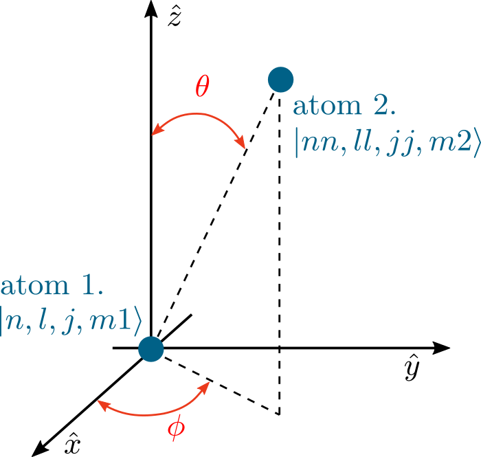
Relative orientation of the two atoms can be described with two polar angles \(\theta\) and \(\phi\) giving polar and azimuth angle. The \(\hat{z}\) axis is here specified relative to the laser driving. For circularly polarized laser light, this is the direction of laser beam propagation. For linearly polarized light, this is the plane of the electric field polarization, perpendicular to the laser direction.
Internal coupling between the two atoms in \(|n,l,j,m_1\rangle\) and \(|nn,ll,jj,m_2\rangle\) is calculated easily for the two atoms positioned so that \(\theta = 0\), and for other angles wignerD matrices are used to change a basis and perform calculation in the basis where couplings are more clearly seen.
Overview
PairStateInteractions Methods
PairStateInteractions.defineBasis(theta, ...) |
Finds relevant states in the vicinity of the given pair-state |
PairStateInteractions.getC6perturbatively(...) |
Calculates \(C_6\) from second order perturbation theory. |
PairStateInteractions.getLeRoyRadius() |
Returns Le Roy radius for initial pair-state. |
PairStateInteractions.diagonalise(rangeR, ...) |
Finds eigenstates in atom pair basis. |
PairStateInteractions.plotLevelDiagram([...]) |
Plots pair state level diagram |
PairStateInteractions.showPlot([interactive]) |
Shows level diagram printed by |
PairStateInteractions.exportData(fileBase[, ...]) |
Exports PairStateInteractions calculation data. |
PairStateInteractions.getC6fromLevelDiagram(...) |
Finds \(C_6\) coefficient for original pair state. |
PairStateInteractions.getC3fromLevelDiagram(...) |
Finds \(C_3\) coefficient for original pair state. |
PairStateInteractions.getVdwFromLevelDiagram(...) |
Finds \(r_{\rm vdW}\) coefficient for original pair state. |
StarkMapResonances Methods
StarkMapResonances.findResonances(nMin, ...) |
Finds near-resonant dipole-coupled pair-states |
StarkMapResonances.showPlot([interactive]) |
Plots initial state Stark map and its dipole-coupled resonances |
Detailed documentation
Pair-state basis level diagram calculations
Calculates Rydberg spaghetti of level diagrams, as well as pertubative C6 and similar properties. It also allows calculation of Foster resonances tuned by DC electric fields.
Example
Calculation of the Rydberg eigenstates in pair-state basis for Rubidium in the vicinity of the \(|60~S_{1/2}~m_j=1/2,~60~S_{1/2}~m_j=1/2\rangle\) state. Colour highlights coupling strength from state \(6~P_{1/2}~m_j=1/2\) with \(\pi\) (\(q=0\)) polarized light. eigenstates:
from arc import *
calc1 = PairStateInteractions(Rubidium(), 60, 0, 0.5, 60, 0, 0.5,0.5, 0.5)
calc1.defineBasis( 0., 0., 4, 5,10e9)
# optionally we can save now results of calculation for future use
saveCalculation(calc1,"mycalculation.pkl")
calculation1.diagonalise(linspace(1,10.0,30),250,progressOutput = True,drivingFromState=[6,1,0.5,0.5,0])
calc1.plotLevelDiagram()
calc1.ax.set_xlim(1,10)
calc1.ax.set_ylim(-2,2)
calc1.showPlot()
-
class
arc.calculations_atom_pairstate.PairStateInteractions(atom, n, l, j, nn, ll, jj, m1, m2, interactionsUpTo=1)[source]¶ Calculates Rydberg level diagram (spaghetti) for the given pair state
Initializes Rydberg level spaghetti calculation for the given atom in the vicinity of the given pair state. For details of calculation see Ref. [1]. For a quick start point example see interactions example snippet.
Parameters: - atom (
AlkaliAtom) – ={alkali_atom_data.Lithium6,alkali_atom_data.Lithium7,alkali_atom_data.Sodium,alkali_atom_data.Potassium39,alkali_atom_data.Potassium40,alkali_atom_data.Potassium41,alkali_atom_data.Rubidium85,alkali_atom_data.Rubidium87,alkali_atom_data.Caesium} Select the alkali metal for energy level diagram calculation - n (int) – principal quantum number for the first atom
- l (int) – orbital angular momentum for the first atom
- j (float) – total angular momentum for the first atom
- nn (int) – principal quantum number for the second atom
- ll (int) – orbital angular momentum for the second atom
- jj (float) – total angular momentum for the second atom
- m1 (float) – projection of the total angular momentum on z-axis for the first atom
- m2 (float) – projection of the total angular momentum on z-axis for the second atom
- interactionsUpTo (int) – Optional. If set to 1, includes only dipole-dipole interactions. If set to 2 includes interactions up to quadrupole-quadrupole. Default value is 1.
References
[1] T. G Walker, M. Saffman, PRA 77, 032723 (2008) https://doi.org/10.1103/PhysRevA.77.032723 Examples
Advanced interfacing of pair-state interactions calculations (PairStateInteractions class). This is an advanced example intended for building up extensions to the existing code. If you want to directly access the pair-state interaction matrix, constructed by
defineBasis, you can assemble it easily from diagonal part (stored inmatDiagonal) and off-diagonal matrices whose spatial dependence is \(R^{-3},R^{-4},R^{-5}\) stored in that order inmatR. Basis states are stored inbasisStatesarray.>>> from arc import * >>> calc = PairStateInteractions(Rubidium(), 60,0,0.5, 60,0,0.5, 0.5,0.5,interactionsUpTo = 1) >>> # theta=0, phi = 0, range of pqn, range of l, deltaE = 25e9 >>> calc.defineBasis(0 ,0 , 5, 5, 25e9, progressOutput=True) >>> # now calc stores interaction matrix and relevant basis >>> # we can access this directly and generate interaction matrix >>> # at distance rval : >>> rval = 4 # in mum >>> matrix = calc.matDiagonal >>> rX = (rval*1.e-6)**3 >>> for matRX in self.matR: >>> matrix = matrix + matRX/rX >>> rX *= (rval*1.e-6) >>> # matrix variable now holds full interaction matrix for >>> # interacting atoms at distance rval calculated in >>> # pair-state basis states can be accessed as >>> basisStates = calc.basisStates
-
atom= None¶ atom type
-
basisStates= None¶ List of pair-states for calculation. In the form [[n1,l1,j1,mj1,n2,l2,j2,mj2], ...]. Each state is an array [n1,l1,j1,mj1,n2,l2,j2,mj2] corresponding to \(|n_1,l_1,j_1,m_{j1},n_2,l_2,j_2,m_{j2}\rangle\) state. Calculated by
defineBasis.
-
channel= None¶ states relevant for calculation, defined in J basis (not resolving \(m_j\). Used as intermediary for full interaction matrix calculation by
defineBasis.
-
coupling= None¶ List of matrices defineing coupling strengths between the states in J basis (not resolving \(m_j\) ). Basis is given by
channel. Used as intermediary for full interaction matrix calculation bydefineBasis.
-
defineBasis(theta, phi, nRange, lrange, energyDelta, progressOutput=False, debugOutput=False)[source]¶ Finds relevant states in the vicinity of the given pair-state
Finds relevant pair-state basis and calculates interaction matrix. Pair-state basis is saved in
basisStates. Interaction matrix is saved in parts depending on the scaling with distance. Diagonal elementsmatDiagonal, correponding to relative energy defects of the pair-states, don’t change with interatomic separation. Off diagonal elements can depend on distance as \(R^{-3}, R^{-4}\) or \(R^{-5}\), corresponding to dipole-dipole (\(C_3\) ), dipole-qudrupole (\(C_4\) ) and quadrupole-quadrupole coupling (\(C_5\) ) respectively. These parts of the matrix are stored inmatRin that order. I.e.matR[0]stores dipole-dipole coupling (\(\propto R^{-3}\)),matR[0]stores dipole-quadrupole couplings etc.Parameters: - theta (float) – relative orientation of the two atoms (see figure on top of the page)
- phi (float) – relative orientation of the two atoms (see figure on top of the page)
- nRange (int) – how much below and above the given principal quantum number of the pair state we should be looking?
- lrange (int) – what is the maximum angular orbital momentum state that we are including in calculation
- energyDelta (float) – what is maximum energy difference ( \(\Delta E/h\) in Hz) between the original pair state and the other pair states that we are including in calculation
- progressOutput (bool) – optional, False by default. If true, prints information about the progress of the calculation.
- debugOutput (bool) – optional, False by default. If true, similar to progressOutput=True, this will print information about the progress of calculations, but with more verbose output.
See also
alkali_atom_functions.saveCalculationandalkali_atom_functions.loadSavedCalculationfor information on saving intermediate results of calculation for later use.
-
diagonalise(rangeR, noOfEigenvectors, drivingFromState=[0, 0, 0, 0, 0], eigenstateDetuning=0.0, progressOutput=False, debugOutput=False)[source]¶ Finds eigenstates in atom pair basis.
ARPACK (
scipy.sparse.linalg.eigsh) calculation of the noOfEigenvectors eigenvectors closest to the original state. If drivingFromState is specified as [n,l,j,mj,q] coupling between the pair-states and the situation where one of the atoms in the pair state basis is in \(|n,l,j,m_j\rangle\) state due to driving with a laser field that drives \(q\) transition (+1,0,-1 for \(\sigma^-\), \(\pi\) and \(\sigma^+\) transitions respectively) is calculated and marked by the colourmaping these values on the obtained eigenvectors.Parameters: - rangeR (
array) – Array of values for distance between the atoms (in \(\mu\) m) for which we want to calculate eigenstates. - noOfEigenvectors (int) – number of eigen vectors closest to the energy of the original (unperturbed) pair state. Has to be smaller then the total number of states.
- eigenstateDetuning (float, optional) – Default is 0. This specifies detuning from the initial pair-state (in Hz) around which we want to find noOfEigenvectors eigenvectors. This is useful when looking only for couple of off-resonant features.
- drivingFromState ([int,int,float,float,int]) – Optional. State of the one of the atoms from the original pair-state basis from which we try to dribe to the excited pair-basis manifold. By default, program will calculate just contribution of the original pair-state in the eigenstates obtained by diagonalization, and will highlight it’s admixure by colour mapping the obtained eigenstates plot.
- progressOutput (bool) – optional, False by default. If true, prints information about the progress of the calculation.
- debugOutput (bool) – optional, False by default. If true, similar to progressOutput=True, this will print information about the progress of calculations, but with more verbose output.
- rangeR (
-
exportData(fileBase, exportFormat='csv')[source]¶ Exports PairStateInteractions calculation data.
Only supported format (selected by default) is .csv in a human-readable form with a header that saves details of calculation. Function saves three files: 1) filebase _r.csv; 2) filebase _energyLevels 3) filebase _highlight
For more details on the format, see header of the saved files.
Parameters: - filebase (string) – filebase for the names of the saved files without format extension. Add as a prefix a directory path if necessary (e.g. saving outside the current working directory)
- exportFormat (string) – optional. Format of the exported file. Currently only .csv is supported but this can be extended in the future.
-
getC3fromLevelDiagram(rStart, rStop, showPlot=False, minStateContribution=0.0, resonantBranch=1)[source]¶ Finds \(C_3\) coefficient for original pair state.
Function first finds for each distance in the range [rStart , rStop] the eigen state with highest contribution of the original state. One can set optional parameter minStateContribution to value in the range [0,1), so that function finds only states if they have contribution of the original state that is bigger then minStateContribution.
Once original pair-state is found in the range of interatomic distances, from smallest rStart to the biggest rStop, function will try to perform fitting of the corresponding state energy \(E(R)\) at distance \(R\) to the function \(A+C_3/R^3\) where \(A\) is some offset.
Parameters: - rStart (float) – smallest inter-atomic distance to be used for fitting
- rStop (float) – maximum inter-atomic distance to be used for fitting
- showPlot (bool) – If set to true, it will print the plot showing fitted energy level and the obtained best fit. Default is False
- minStateContribution (float) – valid values are in the range [0,1). It specifies minimum amount of the original state in the given energy state necessary for the state to be considered for the adiabatic continuation of the original unperturbed pair state.
- resonantBranch (int) – optional, default +1. For resonant interactions we have two branches with identical state contributions. In this case, we will select only positively detuned branch (for resonantBranch = +1) or negatively detuned branch (fore resonantBranch = -1) depending on the value of resonantBranch optional parameter
Returns: \(C_3\) measured in \(\text{GHz }\mu\text{m}^6\) on success; If unsuccessful returns False.
Return type: Note
In order to use this functions, highlighting in
diagonaliseshould be based on the original pair state contribution of the eigenvectors (that this, drivingFromState parameter should not be set, which corresponds to drivingFromState = [0,0,0,0,0]).
-
getC6fromLevelDiagram(rStart, rStop, showPlot=False, minStateContribution=0.0)[source]¶ Finds \(C_6\) coefficient for original pair state.
Function first finds for each distance in the range [ rStart , rStop ] the eigen state with highest contribution of the original state. One can set optional parameter minStateContribution to value in the range [0,1), so that function finds only states if they have contribution of the original state that is bigger then minStateContribution.
Once original pair-state is found in the range of interatomic distances, from smallest rStart to the biggest rStop, function will try to perform fitting of the corresponding state energy \(E(R)\) at distance \(R\) to the function \(A+C_6/R^6\) where \(A\) is some offset.
Parameters: - rStart (float) – smallest inter-atomic distance to be used for fitting
- rStop (float) – maximum inter-atomic distance to be used for fitting
- showPlot (bool) – If set to true, it will print the plot showing fitted energy level and the obtained best fit. Default is False
- minStateContribution (float) – valid values are in the range [0,1). It specifies minimum amount of the original state in the given energy state necessary for the state to be considered for the adiabatic continuation of the original unperturbed pair state.
Returns: \(C_6\) measured in \(\text{GHz }\mu\text{m}^6\) on success; If unsuccessful returns False.
Return type: Note
In order to use this functions, highlighting in
diagonaliseshould be based on the original pair state contribution of the eigenvectors (that this, drivingFromState parameter should not be set, which corresponds to drivingFromState = [0,0,0,0,0]).
-
getC6perturbatively(theta, phi, nRange, energyDelta)[source]¶ Calculates \(C_6\) from second order perturbation theory.
This calculation is faster then full diagonalization, but it is valid only far from the so called spaghetti region that occurs when atoms are close to each other. In that region multiple levels are strongly coupled, and one needs to use full diagonalization.
See pertubative C6 calculations example snippet.
Parameters: - theta (float) – orientation of inter-atomic axis with respect to quantization axis (\(z\)) in Euler coordinates (measured in units of radian)
- phi (float) – orientation of inter-atomic axis with respect to quantization axis (\(z\)) in Euler coordinates (measured in units of radian)
- nRange (int) – how much below and above the given principal quantum number of the pair state we should be looking
- energyDelta (float) – what is maximum energy difference ( \(\Delta E/h\) in Hz) between the original pair state and the other pair states that we are including in calculation
Returns: \(C_6\) measured in \(\text{GHz }\mu\text{m}^6\)
Return type: Example
If we want to quickly calculate \(C_6\) for two Rubidium atoms in state \(62 D_{3/2} m_j=3/2\), positioned in space along the shared quantization axis:
from arc import *
calculation = PairStateInteractions(Rubidium(), 62, 2, 1.5, 62, 2, 1.5, 1.5, 1.5)
c6 = calculation.getC6pertubatively(0,0, 5, 25e9)
print "C_6 = %.0f GHz (mu m)^6" % c6
Which returns:
C_6 = 767 GHz (mu m)^6
Quick calculation of angular anisotropy of for Rubidium \(D_{2/5},m_j=5/2\) states:
# Rb 60 D_{2/5}, mj=2.5 , 60 D_{2/5}, mj=2.5 pair state
calculation1 = PairStateInteractions(Rubidium(), 60, 2, 2.5, 60, 2, 2.5, 2.5, 2.5)
# list of atom orientations
thetaList = np.linspace(0,pi,30)
# do calculation of C6 pertubatively for all atom orientations
c6 = []
for theta in thetaList:
    value = calculation1.getC6pertubatively(theta,0,5,25e9)
    c6.append(value)
    print ("theta = %.2f * pi       C6 = %.2f GHz  mum^6" % (theta/pi,value))
# plot results
plot(thetaList/pi,c6,"b-")
title("Rb, pairstate  60 $D_{5/2},m_j = 5/2$, 60 $D_{5/2},m_j = 5/2$")
xlabel(r"$\Theta /\pi$")
ylabel(r"$C_6$ (GHz $\mu$m${}^6$")
show()
-
getLeRoyRadius()[source]¶ Returns Le Roy radius for initial pair-state.
Le Roy radius [2] is defined as \(2(\langle r_1^2 \rangle^{1/2} + \langle r_2^2 \rangle^{1/2})\), where \(r_1\) and \(r_2\) are electron coordinates for the first and the second atom in the initial pair-state. Below this radius, calculations are not valid since electron wavefunctions start to overlap.
Returns: LeRoy radius measured in \(\mu m\) Return type: float References
[2] R.J. Le Roy, Can. J. Phys. 52, 246 (1974) http://www.nrcresearchpress.com/doi/abs/10.1139/p74-035
-
getVdwFromLevelDiagram(rStart, rStop, showPlot=False, minStateContribution=0.0)[source]¶ Finds \(r_{\rm vdW}\) coefficient for original pair state.
Function first finds for each distance in the range [rStart,`rStop`] the eigen state with highest contribution of the original state. One can set optional parameter minStateContribution to value in the range [0,1), so that function finds only states if they have contribution of the original state that is bigger then minStateContribution.
Once original pair-state is found in the range of interatomic distances, from smallest rStart to the biggest rStop, function will try to perform fitting of the corresponding state energy \(E(R)\) at distance \(R\) to the function \(A+B\frac{1-\sqrt{1+(r_{\rm vdW}/r)^6}}{1-\sqrt{1+r_{\rm vdW}^6}}\)
where \(A\) and \(B\) are some offset.Parameters: - rStart (float) – smallest inter-atomic distance to be used for fitting
- rStop (float) – maximum inter-atomic distance to be used for fitting
- showPlot (bool) – If set to true, it will print the plot showing fitted energy level and the obtained best fit. Default is False
- minStateContribution (float) – valid values are in the range [0,1). It specifies minimum amount of the original state in the given energy state necessary for the state to be considered for the adiabatic continuation of the original unperturbed pair state.
Returns: \(r_{\rm vdW}\) measured in \(\mu\text{m}\) on success; If unsuccessful returns False.
Return type: Note
In order to use this functions, highlighting in
diagonaliseshould be based on the original pair state contribution of the eigenvectors (that this, drivingFromState parameter should not be set, which corresponds to drivingFromState = [0,0,0,0,0]).
-
interactionsUpTo= None¶ ” Specifies up to which approximation we include in pair-state interactions. By default value is 1, corresponding to pair-state interactions up to dipole-dipole coupling. Value of 2 is also supported, corresponding to pair-state interactions up to quadrupole-quadrupole coupling.
-
j= None¶ pair-state definition – total angular momentum of the first atom
-
jj= None¶ pair-state definition – total angular momentum of the second atom
-
l= None¶ pair-state definition – orbital angular momentum of the first atom
-
ll= None¶ pair-state definition – orbital angular momentum of the second atom
-
m1= None¶ pair-state definition – projection of the total ang. momentum for the first atom
-
m2= None¶ pair-state definition – projection of the total angular momentum for the second atom
-
matDiagonal= None¶ Part of interaction matrix in pair-state basis that doesn’t depend on inter-atomic distance. E.g. diagonal elements of the interaction matrix, that describe energies of the pair states in unperturbed basis, will be stored here. Basis states are stored in
basisStates. Calculated bydefineBasis.
-
matR= None¶ Stores interaction matrices in pair-state basis that scale as \(1/R^3\), \(1/R^4\) and \(1/R^5\) with distance in
matR[0],matR[1]andmatR[2]respectively. These matrices correspond to dipole-dipole ( \(C_3\)), dipole-quadrupole ( \(C_4\)) and quadrupole-quadrupole ( \(C_5\)) interactions coefficients. Basis states are stored inbasisStates. Calculated bydefineBasis.
-
matrixElement= None¶ matrixElement[i] gives index of state in
channelbasis (that doesn’t resolvem_jstates), for the given index i of the state inbasisStates( \(m_j\) resolving) basis.
-
n= None¶ pair-state definition – principal quantum number of the first atom
-
nn= None¶ pair-state definition – principal quantum number of the second atom
-
originalPairStateIndex= None¶ index of the original n,l,j,m1,nn,ll,jj,m2 pair-state in the
basisStatesbasis.
-
plotLevelDiagram(highlightColor='red')[source]¶ Plots pair state level diagram
Call
showPlotif you want to display a plot afterwards.Parameters: highlightColor (string) – optional, specifies the colour used for state highlighting
-
savePlot(filename='PairStateInteractions.pdf')[source]¶ Saves plot made by
plotLevelDiagramParameters: filename ( str, optional) – file location where the plot should be saved
-
showPlot(interactive=True)[source]¶ Shows level diagram printed by
PairStateInteractions.plotLevelDiagramBy default, it will output interactive plot, which means that clicking on the state will show the composition of the clicked state in original basis (dominant elements)
Parameters: interactive (bool) – optional, by default it is True. If true, plotted graph will be interactive, i.e. users can click on the state to identify the state composition Note
interactive=True has effect if the graphs are explored in usual matplotlib pop-up windows. It doesn’t have effect on inline plots in Jupyter (IPython) notebooks.
- atom (
-
class
arc.calculations_atom_pairstate.StarkMapResonances(atom1, state1, atom2, state2)[source]¶ Calculates pair state Stark maps for finding resonances
Tool for finding conditions for Foster resonances. For a given pair state, in a given range of the electric fields, looks for the pair-state that are close in energy and coupled via dipole-dipole interactions to the original pair-state.
See Stark resonances example snippet.
Parameters: - atom (
AlkaliAtom) –={
alkali_atom_data.Lithium6,alkali_atom_data.Lithium7,alkali_atom_data.Sodium,alkali_atom_data.Potassium39,alkali_atom_data.Potassium40,alkali_atom_data.Potassium41,alkali_atom_data.Rubidium85,alkali_atom_data.Rubidium87,alkali_atom_data.Caesium}the first atom in the pair-state - state1 ([int,int,float,float]) – specification of the state of the first state as an array of values \([n,l,j,m_j]\)
- atom –
={
alkali_atom_data.Lithium6,alkali_atom_data.Lithium7,alkali_atom_data.Sodium,alkali_atom_data.Potassium39,alkali_atom_data.Potassium40,alkali_atom_data.Potassium41,alkali_atom_data.Rubidium85,alkali_atom_data.Rubidium87,alkali_atom_data.Caesium}the second atom in the pair-state - state2 ([int,int,float,float]) – specification of the state of the first state as an array of values \([n,l,j,m_j]\)
Note
In checking if certain state is dipole coupled to the original state, only the highest contributing state is checked for dipole coupling. This should be fine if one is interested in resonances in weak fields. For stronger fields, one might want to include effect of coupling to other contributing base states.
-
findResonances(nMin, nMax, maxL, eFieldList, energyRange=[-5000000000.0, 5000000000.0], progressOutput=False)[source]¶ Finds near-resonant dipole-coupled pair-states
For states in range of principal quantum numbers [nMin,`nMax`] and orbital angular momentum [0,`maxL`], for a range of electric fields given by eFieldList function will find near-resonant pair states.
Only states that are in the range given by energyRange will be extracted from the pair-state Stark maps.
Parameters: - nMin (int) – minimal principal quantum number of the state to be included in the StarkMap calculation
- nMax (int) – maximal principal quantum number of the state to be included in the StarkMap calculation
- maxL (int) – maximum value of orbital angular momentum for the states to be included in the calculation
- eFieldList ([float]) – list of the electric fields (in V/m) for which to calculate level diagram (StarkMap)
- energyRange ([float,float]) – optinal argument. Minimal and maximal energy of that some dipole-coupled state should have in order to keep it in the plot (in units of Hz). By default it finds states that are \(\pm 5\) GHz
- atom (