Below is the list of extension modules for advanced ARC calculations,
contributed by the research community. When using advanced extension modules
for ARC please cite *both* original ARC paper *and* paper that introduced
extension.
Calculates lifetime of atomic population taking into account redistribution of population to other states under spontaneous and black body induced transitions.
getPopulationLifetime(atom, n, l, j, temperature=0, includeLevelsUpTo=0, period=1, plotting=1, thresholdState=False, detailedOutput=False)[source]#
Calculates lifetime of atomic population taking into account
redistribution of population to other states under spontaneous and
black body induced transitions.
It simulates the time evolution of a system in which all the states,
from the fundamental one to the highest state which you want to include,
are taken into account.
The orbital angular momenta taken into account are only S,P,D,F.
This function is based on getStateLifetime but it takes into account
the re-population processess due to BBR-induced transitions.
For this reason lifetimes of Rydberg states are slightly longer
than those returned by getStateLifetime up to 5-10%.
This function creates a .txt file, plots the time evolution of the
population of the Rydberg states and yields the lifetime values by using
the fitting method from Ref. 1 .
Contributed by: Alessandro Greco (alessandrogreco08 at gmail dot com),
Dipartimento di Fisica E. Fermi, Università di Pisa, Largo Bruno Pontecorvo 3, 56127 Pisa, Italy.
The simulations have been compared with experimental data 2 .
M. Archimi, C. Simonelli, L. Di Virgilio, A. Greco,
M. Ceccanti, E. Arimondo, D. Ciampini, I. I. Ryabtsev, I. I. Beterov,
and O. Morsch, Phys. Rev. A100, 030501(R) (2019)
https://doi.org/10.1103/PhysRevA.100.030501
Some definitions:
What are the ensemble, the support, the ground?
According to https://arxiv.org/abs/1907.01254
The sum of the populations of every state which is detected as Rydberg state
(above the threshold state which must be set) is called ensemble
The sum of the populations of every state which is detected as Rydberg state,
without the target state, is called support
The sum of the populations of every state which cannot be detected as Rydberg state
(under the threshold state which must be set) is called groundgammaTargetSpont is the rate which describes transitions
from Target State towards all the levels under the threshold
state, i.e. Ground State
gammaTargetBBR is the rate which describes transitions towards all
the levels above the threshold state, i.e. Support State
gammaSupporSpont is the rate which describes transitions from the
Support State towards all the levels under the threshold state,
i.e. Ground State
gammaSupportBBR is the rate which describes transitions from
upport State towards all the levels above the threshold state,
i.e. Target State)
Parameters
n (int) – principal quantum number of the state whose population lifetime
we are calculating, it’s called the Target state and its color is
green in the plot.
l (int) – orbital angular momentum number of the state whose population lifetime
we are calculating, it’s called the Target state and its color is
green in the plot.
j (float) – total angular momentum of the state whose population lifetime
we are calculating, it’s called the Target state and its color is
green in the plot.
temperature (float) – Temperature at which the atom environment
is, measured in K. If this parameter is non-zero, user has
to specify transitions up to which state (due to black-body
decay) should be included in calculation.
includeLevelsUpTo (int) – At non zero temperatures,
this specifies maximum principal quantum number of the state
to which black-body induced transitions will be included.
Minimal value of the parameter in that case is =`n+1
period – Specifies the period that you want to consider for
the time evolution, in microseconds.
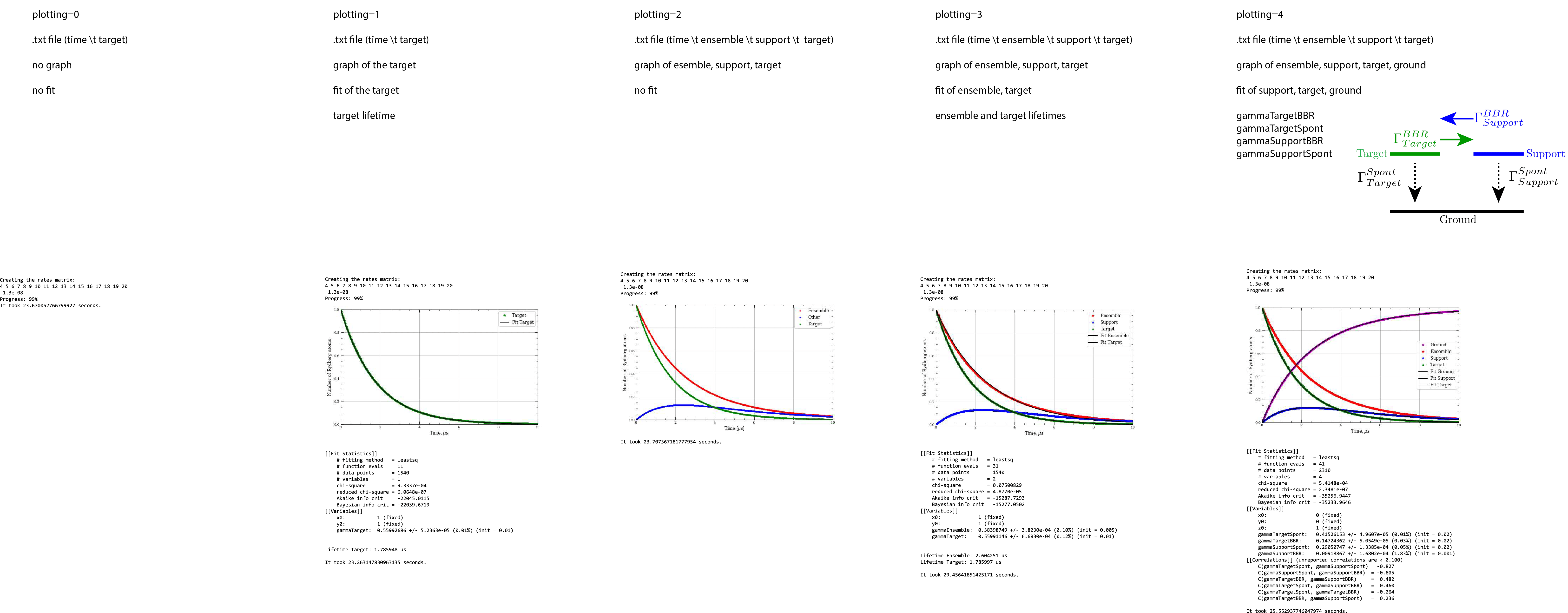
plotting (int) – optional. It is set to 1 by default. The options are
(see also image at the bottom of documentation):
plotting=0 no plot;
plotting=1 plots the population of the target (n,l,j) state
with its fit and it yields the value of the target lifetime
in microseconds;
plotting=2 plots the whole system (Ensemble, Support, Target),
no fit;
plotting=3 plots the whole system (Ensemble, Support, Target)
and it fits the Ensemble and Target curves, it yields the values
of the Ensemble lifetime and Target lifetime in microseconds;
plotting=4 it plots the whole system (Ensemble, Support, Target) +
the Ground (which is the complementary of the ensemble).
It considers the whole system like a three-level model (Ground
State, Support State, Target State) and yields four transition
rates.
thresholdState (int) – optional. It specifies the principal quantum
number n of the lowest state (it’s referred to S state!) which is
detectable by your experimental apparatus, it directly modifies
the Ensemble and the Support (whose colors are red and blue
respectively in the plot). It is necessary to define a threshold
state if plotting = 2, 3 or 4 has been selected. It is not necessary
to define a threshold state if plotting = 0 or 1 has been selected.
detailedOutput=True – optional. It writes a .txt file with the time
evolution of all the states. It is set to false by default.
(The first column is the time, the other are the population of all
the states. The order is time, nS, nP0.5, nP1.5, nD1.5, nD2.5,
nF2.5, nF3.5, and n is ordered from the lowest state to the highest one.
For example: time, 4S, 5S ,6S ,ecc… includeLevelsUpToS, 4P0.5,
5P0.5, 6P0.5, ecc… includeLevelsUpToP0.5, 4P1.5, 5P1.5, 6P1.5, ecc…)
Returns
Plots and a .txt file.
plotting = 0,1 create a .txt file with two coloumns
(time t target population);
plotting = 2,3,4 create a .txt file with four coloumns
(time t ensemble population t support population t target population)