[1]:
%matplotlib inline
[2]:
%load_ext line_profiler
[3]:
import matplotlib.pyplot as plt
import numpy as np
AC Stark Maps#
This notebook contains a primer on how to generate Stark maps of Rydberg states when driven by an AC electric field. Presently, only two types of solvers are implemented:
Shirley’s Time-Independent Floquet Hamiltonian
The approximate RWA-model, which assumes a sum of 2-level systems
Potential extensions of this functionality could include:
Two (or more) simultaneous frequenices via Shirley’s method
Time-dependent integration of the Floquet Hamiltonian’s propagator
Including optically-coupled states not in the Rydberg manifold
Shirley’s Time-Independent Floquet Hamiltonian#
The problem of solving for AC Stark shifts in a large manifold of Rydberg states that can couple to a single RF readily lends itself to a Floquet treatment. Beginning with the time-dependent Shrödinger equation
we assume that the time-dependent perturbation to the bare Hamiltonian is periodic in time such that \(\omega_{rf}\tau = 2\pi\) and \(V(t+\tau) = V(t)\). Under this assumption, solutions to the Shrödinger equation will be periodic as well:
where \(\epsilon\) are known as quasi-energies and \(\Phi(t+\tau) = \Phi(t)\) represent periodic functions for the drive frequency.
We can define the basis in terms of the basis of \(H_0\) and the Fourier vectors as \(|\alpha\rangle\) and \(|n\rangle\), respectively. The Hamiltonian and wave vectors, in this basis, are defined as
where \(H^{[n]}\) represents the \(n\)th-order component of the Fourier expansion of the Hamiltonian.
By subsitution of the quantities into the Shrödinger equation, we can produce an infinite-dimension eigenvalue equation that is time-independent.
where \(H_F\) is block tri-diagonal with elements
Finding the eigenvalues and eigenvectors of this Shirley Floquet Hamiltonian allows us to determine the steady-state basis in the presence of the RF field. Comparing how the energy levels have changed relative to \(H_0\) gives the AC Stark shifts.
Using the eigvectors and eigenvalues of \(H_F\), we can also contruct the time-propagation operator \(U(t,t_0)\), allowing simple calculations of transition probabilities.
The probability to go from state \(\alpha\) to state \(\beta\), assuming all population starts in state \(\alpha\) is given by
When comparing with experimental values, it is often advantageous to average over some of the time-dependence in this probability. To begin, the initial phase of the drive is often not controlled in CW experiments, so one should average over \(t\) while holding \(t-t_0\) fixed to get the time-dependent transition probability as a function of \(\Delta t\).
To obtain the long-time averaged transition probability, one must also integrate over \(t-t_0\). Assuming the integration time is much longer than any non-zero difference \(1/(\epsilon_{\alpha m}-\epsilon_{\beta n})\), one obtains:
This theory is described in more detail by Shirley, Phys. Rev. 138 B979 (1965), Chu, Adv in At and Mol Phys 21 (1985) and the application of this method to Rydberg atoms is shown in Meyer et. al. J Phys B 53 034001 (2020).
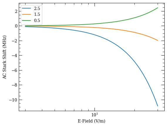
Example AC Stark Map using Shirley’s Floquet Method#
This example calculates the steady-state Stark shifts of the \(|56D_{5/2}\rangle\) state when driven by a relatively weak far-from resonance field of 1.72 GHz with a linear polarization. It calculates the independent response of each available \(m_J\) of the target state.
[4]:
from arc import Rubidium85, ShirleyMethod
[5]:
atom = Rubidium85()

g = [5, 0, 0.5]
i = [5, 1, 1.5]
t = [56, 2, 2.5]

mjs = [2.5, 1.5, 0.5]

nwin = 10
lmax = 20

q = 0
[6]:
Esteps = 600
dBRange = 20  # calculate range spanning 20 dB of RF power
Emax = 30  # V/m
Emin = Emax * 10 ** (-dBRange / 20)
Efields = np.linspace(Emin, Emax, Esteps)

freq = 1.72e9  # in Hz, of the RF field
Given the field is very far-detuned, the resulting Stark shifts are fairly small and allow a reduction of the basis of Rydberg states in the calculation to just dipole-allowed transitions. This greatly speeds up the calculation.
[7]:
results = {}
for mj in mjs:
    m = ShirleyMethod(atom)
    m.defineBasis(
        *t,
        mj,
        q,
        t[0] - nwin,
        t[0] + nwin + 1,
        lmax,
        edN=1,
        progressOutput=False,
        debugOutput=False,
    )
    m.defineShirleyHamiltonian(fn=1)
    m.diagonalise(Efields, freq, progressOutput=True)
    results[mj] = -m.targetShifts * 1e-6  # get results in MHz
Finding eigenvectors...
Finding eigenvectors...
Finding eigenvectors...
100%
[8]:
fig, ax = plt.subplots(1)

for mj, result in results.items():
    ax.plot(Efields, result, label=f"{mj:.1f}")

ax.legend()
ax.set_xscale("log")
ax.set_xlabel("E-Field (V/m)")
ax.set_ylabel("AC Stark Shift (MHz)")
[8]:
Text(0, 0.5, 'AC Stark Shift (MHz)')
The ACStarkMap object saves more information about the solves than just the target state shifts. It also saves the full eigenvalues and eigenvectors from the diagonalisation of the Shirley Hamiltonian.
It will also calculate the long-time averaged transition probability for an atom to go from the target state to any state in the basis (see Eq. 25 of Chu, Adv in At and Mol Phys 21 (1985)):
[9]:
print(f"For the mJ = {m.mj:.1f} calculation")
print(f"For f = {freq*1e-9:.2f} GHz")
print(f"For E = {Efields[-1]:.1f} V/m")

indMaxProb = m.transProbs[-1].argmax()
print(
    f"State with largest overlap with the target state is: {m.basisStates[indMaxProb]}"
)
For the mJ = 0.5 calculation
For f = 1.72 GHz
For E = 30.0 V/m
State with largest overlap with the target state is: [56, 2, 2.5, 0.5]
Given the small shifts and far-detuned field, it is expected that little population would be driven to another state.
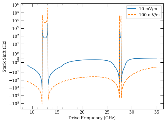
Example AC Stark Map versus Frequency#
Here we calculate Stark shifts of the same target state, but over a range of drive frequencies with two distinct amplitudes.
Note that the drive frequencies cover four distinct resonances as well as large regions where the drive is far from all resonances. Smoothly handling these transitions is the power of a Floquet approach to these types of calculations.
[10]:
atom = Rubidium85()

g = [5, 0, 0.5]
i = [5, 1, 1.5]
t = [56, 2, 2.5]

mjs = [2.5, 1.5, 0.5]

nwin = 10
lmax = 20

q = 0
[11]:
Efields = np.array([0.01, 0.1])

freqs = np.linspace(9e9, 35e9, 600)
[12]:
calc = ShirleyMethod(atom)
calc.defineBasis(
    *t,
    mj,
    q,
    t[0] - nwin,
    t[0] + nwin + 1,
    lmax,
    edN=1,
    progressOutput=False,
    debugOutput=False,
)
calc.defineShirleyHamiltonian(fn=1)
calc.diagonalise(Efields, freqs, progressOutput=True)
Finding eigenvectors...
100%
[13]:
calc.targetShifts.shape
[13]:
(2, 600)
[14]:
fig, ax = plt.subplots(1)

ax.plot(freqs * 1e-9, calc.targetShifts[0], label=f"{Efields[0]*1e3:.0f} mV/m")
ax.plot(
    freqs * 1e-9, calc.targetShifts[1], "--", label=f"{Efields[1]*1e3:.0f} mV/m"
)

ax.legend()
ax.set_yscale("symlog")
ax.set_xscale("linear")

ax.set_xlabel("Drive Frequency (GHz)")
ax.set_ylabel("Stark Shift (Hz)")
[14]:
Text(0, 0.5, 'Stark Shift (Hz)')
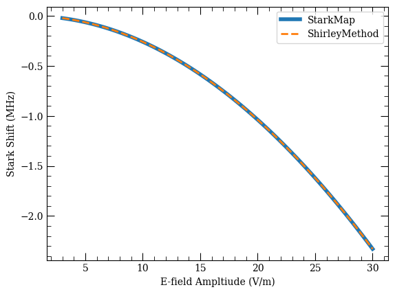
Comparison with StarkMap#
For very low frequency fields that are far-detuned from all resonances, Shirley’s method will reproduce the results from ARC’s StarkMap, differing only by a factor of \(\sqrt{2}\). In other words, the following two approaches give the same result:
DC Stark Shift with the rms field amplitude
AC Stark Shift with the field amplitude
Below we show the Stark Map calculation using both methods for a drive frequency of 50 MHz.
[15]:
from arc import StarkMap
[16]:
atom = Rubidium85()

g = [5, 0, 0.5]
i = [5, 1, 1.5]
t = [56, 2, 2.5]

mj = 0.5

nwin = 10
lmax = 20

q = 0
[17]:
Efields = np.linspace(3, 30, 100)
freq = 50e6
DC Stark Calculation#
[18]:
calc_dc = StarkMap(atom)
[19]:
calc_dc.defineBasis(
    *t, mj, t[0] - nwin, t[0] + nwin + 1, lmax, progressOutput=True
)
Found  861  states.
Generating matrix...
100%
[19]:
0
Note that the RF field amplitude is manually changed to the rms amplitude here. When the RF frequency is faster than the atomic response, the atoms will only see the rms field amplitude, not the full peak-to-peak amplitude that is implicitely assumed by the DC calculation.
[20]:
%%time
calc_dc.diagonalise(Efields / np.sqrt(2), progressOutput=True)
Finding eigenvectors...
100%

CPU times: total: 1min 11s
Wall time: 12 s
AC Stark Calculation#
[21]:
calc_ac = ShirleyMethod(atom)
[22]:
calc_ac.defineBasis(
    *t, mj, q, t[0] - nwin, t[0] + nwin + 1, lmax, progressOutput=True
)
calc_ac.defineShirleyHamiltonian(fn=1)
Found  861  states.
Generating matrix...
100%
Energies and Couplings Generated
Note that the Shirley calculation is significantly slower than the DC StarkMap calculation despite having the same number of basis states. This is because Shirley’s Floquet Hamiltonian is actually three times larger (\(3\times861=2583\)), making the eigenvalue solves slower.
[23]:
%%time
calc_ac.diagonalise(Efields, freq, progressOutput=True)
Finding eigenvectors...
CPU times: total: 12min 43s
Wall time: 2min 13s
Compare#
[24]:
print(f"Target state zero-field energy {calc_ac.targetEnergy*1e-9:.3f} GHz")
Target state zero-field energy -1101.368 GHz
[25]:
# extracts equivalent of `targetShifts` from `StarkMap` calculation
calc_dc_shifts = (
    calc_ac.targetEnergy * 1e-9 - np.asarray(calc_dc.y)
) * 1e3  # converts to MHz as well
targetEigInd = np.argmin(np.abs(calc_dc_shifts[0]))
calc_dc_targetShifts = calc_dc_shifts[:, targetEigInd]
[26]:
fig, ax = plt.subplots(1)

ax.plot(Efields, calc_dc_targetShifts, lw=4, label="StarkMap")
ax.plot(Efields, calc_ac.targetShifts * 1e-6, "--", lw=2, label="ShirleyMethod")

ax.set_xlabel("E-field Ampltiude (V/m)")
ax.set_ylabel("Stark Shift (MHz)")
ax.legend()
[26]:
<matplotlib.legend.Legend at 0x1e6c8fded60>
Caution when using targetShifts#
The algorithm for determining the target state shift is not fool-proof. This is because the eigensolver returns the eigenstates and eigenvalues as a sorted list. If the order of states changes due to large drive field amplitudes, or the target state moves through an avoided crossing with another state in the basis, the resulting targetShifts, transProbs, and calcCWTransitionProbability calculations are likely to be incorrect.
[27]:
atom = Rubidium85()

g = [5, 0, 0.5]
i = [5, 1, 1.5]
t = [56, 2, 2.5]

mjs = [2.5, 1.5, 0.5]

nwin = 10
lmax = 10

q = 0
[28]:
Efields = np.geomspace(1e0, 1.2e1, 100)

freq = 12.3e9
[29]:
calc = ShirleyMethod(atom)
calc.defineBasis(
    *t,
    mj,
    q,
    t[0] - nwin,
    t[0] + nwin + 1,
    lmax,
    edN=0,
    progressOutput=False,
    debugOutput=False,
)
calc.defineShirleyHamiltonian(fn=1)
calc.diagonalise(Efields, freq, progressOutput=True)
Finding eigenvectors...
100%
If we plot the targetShifts we see an unphysical discontinuity in the shift.
[30]:
fig, ax = plt.subplots(1)

ax.plot(Efields, calc.targetShifts * 1e-6, "o-")

ax.set_ylim((-2, 90))
ax.set_ylabel("Target Shift (MHz)")
ax.set_xlabel("E-Field (V/m)")
[30]:
Text(0.5, 0, 'E-Field (V/m)')

If we instead plot all of the eigenvalues (with the target state energy subtracted and on the same scale) we see the “discontinuity” is actually due to an avoided crossing.
[31]:
fig, ax = plt.subplots(1)

ax.plot(Efields, (calc.targetEnergy - calc.eigs) * 1e-6, "o-")

ax.set_ylim((-2, 90))
ax.set_ylabel("Target Shift (MHz)")
ax.set_xlabel("E-Field (V/m)")
[31]:
Text(0.5, 0, 'E-Field (V/m)')

RWAStarkShift: Approximating AC Stark Map Calculations#
If the Stark shifts due to the applied field are small, it is generally possible to make simplifying approximations that greatly speed up the calculation.
[32]:
from arc import RWAStarkShift
[33]:
atom = Rubidium85()

g = [5, 0, 0.5]
i = [5, 1, 1.5]
t = [56, 2, 2.5]

mj = 0.5

nwin = 10
lmax = 10

q = 0
[34]:
freqs = np.linspace(-0.5e9, 1.5e9, 400) + 12e9
eField = 0.1  # V/m
This is the full basis solve including any Rydberg state with principle quantum number \(\pm10\) and \(L<10\).
[35]:
%%time

calc_full = ShirleyMethod(atom)
calc_full.defineBasis(
    *t, mj, q, t[0] - nwin, t[0] + nwin + 1, lmax, edN=0, progressOutput=True
)
calc_full.defineShirleyHamiltonian(fn=1)
calc_full.diagonalise(eField, freqs, progressOutput=True)
Found  441  states.
Generating matrix...
100%
Energies and Couplings Generated
Finding eigenvectors...
CPU times: total: 8min 5s
Wall time: 1min 25s
[36]:
fig, ax = plt.subplots(1)

ax.plot(freqs * 1e-9, calc_full.targetShifts * 1e-6)
ax.set_xlabel("RF Frequency (GHz)")
ax.set_ylabel("AC Stark Shift (MHz)")
[36]:
Text(0, 0.5, 'AC Stark Shift (MHz)')

The assymmetric resonances are due to a course grid relative to the resonance widths.
Here is a reduced basis calculation that only includes states with a coupling to the target state that is dipole-allowed via a single photon.
[37]:
%%time

calc_reduced = ShirleyMethod(atom)
calc_reduced.defineBasis(
    *t, mj, q, t[0] - nwin, t[0] + nwin + 1, lmax, edN=1, progressOutput=True
)
calc_reduced.defineShirleyHamiltonian(fn=1)
calc_reduced.diagonalise(eField, freqs, progressOutput=True)
Found  64  states.
Generating matrix...
100%
Energies and Couplings Generated
Finding eigenvectors...
CPU times: total: 7.69 s
Wall time: 2.24 s
[38]:
fig, ax = plt.subplots(1)

ax.plot(freqs * 1e-9, calc_reduced.targetShifts * 1e-6)
ax.set_xlabel("RF Frequency (GHz)")
ax.set_ylabel("AC Stark Shift (MHz)")
[38]:
Text(0, 0.5, 'AC Stark Shift (MHz)')

A significantly faster approximation can be made by simply assuming the 2-level rotating wave approximation result holds for each dipole-allowed transition, with the shift from each state pair being added linearly.
Note that the sign of \(\delta_i\) and the sign in the equation depends on whether the target state is higher or lower in energy than the coupled state.
This method is significantly faster, though certainly limited in its accuracy.
[39]:
%%time

calc_rwa = RWAStarkShift(atom)
calc_rwa.defineBasis(
    *t,
    mj,
    q,
    t[0] - nwin,
    t[0] + nwin + 1,
    lmax,
    edN=1,
    progressOutput=False,
    debugOutput=False,
)
calc_rwa.findDipoleCoupledStates(debugOutput=True)
calc_rwa.makeRWA(eField, freqs)
Found 63 dipole coupled states
Nearest dipole coupled state is detuned by: 12.007 GHz
Calculating RWA Stark Shift approximation with 63 levels
CPU times: total: 1.16 s
Wall time: 1.16 s
[40]:
fig, ax = plt.subplots(1)

ax.plot(freqs * 1e-9, calc_rwa.starkShifts * 1e-6)
ax.set_xlabel("MW Freq (GHz)")
ax.set_ylabel("Stark Shift (GHz)")
[40]:
Text(0, 0.5, 'Stark Shift (GHz)')

Comparing the two approximate methods to the full method shows the relative accuracy.
[41]:
fig, ax = plt.subplots(1)

ax.plot(
    freqs * 1e-9,
    np.abs(
        (calc_full.targetShifts - calc_reduced.targetShifts)
        / calc_full.targetShifts
    )
    * 100,
    label="Reduced Basis",
)
ax.plot(
    freqs * 1e-9,
    np.abs(
        (calc_full.targetShifts - calc_rwa.starkShifts) / calc_full.targetShifts
    )
    * 100,
    label="RWA",
)
ax.set_xlabel("MW Freq (GHz)")
ax.set_ylabel("Fractional Error from full calculation (%)")
ax.legend()
[41]:
<matplotlib.legend.Legend at 0x1e6e3a715b0>

2-level Floquet Analysis#
The below example shows how to construct a 2-level system using specific states.
We will use this simplified system to demonstrate calculations of transition probabilities between states.
[42]:
atom = Rubidium85()
t = [56, 2, 2.5]

mj = 0.5
q = 0
[43]:
m = ShirleyMethod(atom)
m.defineBasis(
    *t,
    mj,
    basisStates=[[56, 2, 2.5, 0.5], [57, 1, 1.5, 0.5]],
    progressOutput=True,
    debugOutput=False,
)
m.defineShirleyHamiltonian(fn=1)
Generating matrix...
100%
Energies and Couplings Generated
[44]:
Efield = 5  # V/m
f0 = 12.0073e9  # Hz

freqs = np.linspace(-1e9, 1e9, 101) + f0
[45]:
m.diagonalise(Efield, freqs, progressOutput=True)
Finding eigenvectors...
100%
Here we plot both the target state shift and the long-time averaged transition probability to be in either state.
[46]:
fig, (ax1, ax2) = plt.subplots(2, sharex=True)

ax1.plot(freqs * 1e-9, m.targetShifts * 1e-6)

ax2.plot(freqs * 1e-9, m.transProbs[:, 0], label="Target State")
ax2.plot(freqs * 1e-9, m.transProbs[:, 1], label="Coupled State")
ax1.set_ylabel("Target State Shift (MHz)")
ax2.set_ylabel("Transition Probability")
ax2.set_xlabel("Drive Frequency (GHz)")
ax2.legend();

We can also calculate the time-dependent transition probabilities, having averaged over the t=0 drive phase. We will see the resulting Rabi flopping between states, which depends on drive amplitude and detuning from resonance.
[47]:
tau = 1 / f0
ts = np.linspace(0, 500 * tau, 200)

t_tp = m.calcTransitionProbability(ts)
[48]:
ifreqs = [40, 49, 50, 55, 70]
fig, axs = plt.subplots(len(ifreqs), sharex=True, figsize=(6, 12), sharey=True)

ax1.set_ylim((0, 1.1))
f = 50
for i, ifr in enumerate(ifreqs):
    axs[i].set_title(
        f"Efield: {Efield:.1f} V/m, Detuning: {(freqs[ifr]-f0)*1e-6:.1f} MHz"
    )
    axs[i].plot(ts / tau, t_tp[:, ifr, :])
    axs[i].plot(ts / tau, t_tp[:, ifr, :].sum(axis=-1), "--", label="sum")

axs[-1].set_xlabel("Time ($1/f_0$)")
[48]:
Text(0.5, 0, 'Time ($1/f_0$)')

[ ]: