ARC Additions: Notebook of new functions and testing / benchmarking to verify parameters and sources#

Goal: Transfer hyperfine atomic physics functions from internal Matlab toolbox to ARC.

Jonathan Pritchard, University of Strathclyde (2020)

[8]:

# Configure Environment

from arc import *

%matplotlib inline
import matplotlib.pyplot as plt
import numpy as np

cs = Cesium()
rb87 = Rubidium87()

Check ARC Parameters for D1/2 and inverted (n+1)P_{1/2,3/2}#

New function A, B = self.getHFSCoefficients(self, n, l, j, s=None) added to return HFS constants in Hz. Refernce [5] and [6] have useful reference info

Hyperfine Structure Functions#

A, B = atom.getHFSCoefficients(n,l,j)

Returns HFS constants in Hz. This is currently using hard-coded values for Cs and Rb, but has been written as a place-holder for adding in a table. Refernce [5] and [6] have useful reference info.

getHFSEnergyShift(j, f, A, B)

Returns HFS Energy shift from centre of mass.

\begin{equation} \Delta E_\mathrm{hfs} = \frac{A}{2}K+B\frac{\frac{3}{2}K(K+1)-2I(I+1)J(J+1)}{2I(2I-1)2J(2J-1)}, \end{equation} where \(K=F(F+1)-I(I+1)-J(J+1)\).

References#

[1] Steck

[2] M. Ortiz and J. Campos, J. Quant. Spectrosc. Radiat. Transfer 26, 107 (1981)

[3] Vasilyev, A. A. and Savukov, I. M. and Safronova, M. S. and Berry, H. G., PRA 66, 020101 (2002)

[4] M. S. Safronova, Carl J. Williams, and Charles W. Clark, PRA 69, 022509 (2004)

[5] D. Feiertag, A. Sahm, and G. zu Putlitz, Z. Phys. 255, 93 (1972)

[6] E. Arrimondo, M. Inguscio and P. Violino, Rev. Mod. Phys. 49, 31 (1977)

[2]:

print("Cs Numbers")
print("==========")
print("State Lifetimes:")
# Lifetime Comparison -->
print(
    "\t[1] : Tau6P1/2 = 34.894(44) ns, ARC = %2.3f ns (%2.2f %% error)"
    % (
        cs.getStateLifetime(6, 1, 0.5) * 1e9,
        (cs.getStateLifetime(6, 1, 0.5) * 1e9 - 34.894) / 34.894 * 100,
    )
)
print(
    "\t[1] : Tau6P3/2 = 30.473(44) ns, ARC = %2.3f ns (%2.2f %% error)"
    % (
        cs.getStateLifetime(6, 1, 1.5) * 1e9,
        (cs.getStateLifetime(6, 1, 1.5) * 1e9 - 30.473) / 30.473 * 100,
    )
)
print(
    "\t[2] : Tau7P1/2 = 155 ns, ARC = %2.3f ns (%2.2f %% error)"
    % (
        cs.getStateLifetime(7, 1, 0.5) * 1e9,
        (cs.getStateLifetime(7, 1, 0.5) * 1e9 - 155) / 155 * 100,
    )
)
print(
    "\t[2] : Tau7P3/2 = 133 ns, ARC = %2.3f ns (%2.2f %% error)"
    % (
        cs.getStateLifetime(7, 1, 1.5) * 1e9,
        (cs.getStateLifetime(7, 1, 1.5) * 1e9 - 133) / 133 * 100,
    )
)
# Matrix Elements
print("Matrix Elements")
r = 4.5003
rm = cs.getReducedMatrixElementJ(6, 0, 0.5, 6, 1, 0.5)
print(
    "\t[1] : <6S1/2||er||6P1/2> = %1.4f, ARC = %2.4f ns (%2.2f %% error)"
    % (r, rm, (rm - r) / r * 100)
)
r = 6.3338
rm = cs.getReducedMatrixElementJ(6, 0, 0.5, 6, 1, 1.5)
print(
    "\t[1] : <6S1/2||er||6P3/2> = %1.4f, ARC = %2.4f ns (%2.2f %% error)"
    % (r, rm, (rm - r) / r * 100)
)
r = 0.2757
rm = cs.getReducedMatrixElementJ(6, 0, 0.5, 7, 1, 0.5)
print(
    "\t[3] : <6S1/2||er||7P1/2> = %1.4f, ARC = %2.4f ns (%2.2f %% error)"
    % (r, rm, (rm - r) / r * 100)
)
r = 0.5856
rm = cs.getReducedMatrixElementJ(6, 0, 0.5, 7, 1, 1.5)
print(
    "\t[3] : <6S1/2||er||7P3/2> = %1.4f, ARC = %2.4f ns (%2.2f %% error)"
    % (r, rm, (rm - r) / r * 100)
)
# Hyperfine Splitting Coefficients
print("Hyperfine Constants")
A, B = cs.getHFSCoefficients(6, 0, 0.5)
omegaQ = 4 * A
print("\t[1] : 6S1/2 A = %1.4f MHz,B = %1.4f MHz" % (A * 1e-6, B * 1e-6))
A, B = cs.getHFSCoefficients(6, 1, 0.5)
print("\t[1] : 6P1/2 A = %1.4f MHz,B = %1.4f MHz" % (A * 1e-6, B * 1e-6))
A, B = cs.getHFSCoefficients(6, 1, 1.5)
print("\t[1] : 6P3/2 A = %1.4f MHz,B = %1.4f MHz" % (A * 1e-6, B * 1e-6))
A, B = cs.getHFSCoefficients(7, 1, 0.5)
print("\t[5] : 7P1/2 A = %1.4f MHz,B = %1.4f MHz" % (A * 1e-6, B * 1e-6))
A, B = cs.getHFSCoefficients(7, 1, 1.5)
print("\t[6] : 7P3/2 A = %1.4f MHz,B = %1.4f MHz" % (A * 1e-6, B * 1e-6))

print("\nVerify getHFSCoefficients(j,f,A,B) using Cs 6P3/2")
A, B = cs.getHFSCoefficients(6, 1, 1.5)
Ehfs = cs.getHFSEnergyShift(1.5, 5, A, B)
print(
    "\t[1] : 6P3/2 F=5: Ehfs = +263.81 MHz --> ARC Ehfs = %f MHz"
    % (Ehfs * 1e-6)
)
Ehfs = cs.getHFSEnergyShift(1.5, 4, A, B)
print(
    "\t[1] : 6P3/2 F=4: Ehfs =  +12.815 MHz --> ARC Ehfs = %f MHz"
    % (Ehfs * 1e-6)
)
Ehfs = cs.getHFSEnergyShift(1.5, 3, A, B)
print(
    "\t[1] : 6P3/2 F=3: Ehfs = -188.44 MHz --> ARC Ehfs = %f MHz"
    % (Ehfs * 1e-6)
)
Ehfs = cs.getHFSEnergyShift(1.5, 2, A, B)
print(
    "\t[1] : 6P3/2 F=2: Ehfs = -339.64 MHz --> ARC Ehfs = %f MHz"
    % (Ehfs * 1e-6)
)


# Clock Frequency
print(
    "\n\t[1] : 6S1/2 Clock Frequency = 9.192631770 GHz --> ARC = %f GHz (%2.2f %% error)"
    % (omegaQ * 1e-9, (omegaQ - 9.192631770e9) / 9.192631770e9 * 100)
)

print("\nRb Numbers")
print("==========")
print("State Lifetimes:")

# Lifetime Comparison -->
print(
    "\t[1] : Tau5P1/2 = 27.70(4) ns, ARC = %2.3f ns (%2.2f %% error)"
    % (
        rb87.getStateLifetime(5, 1, 0.5) * 1e9,
        (rb87.getStateLifetime(5, 1, 0.5) * 1e9 - 27.70) / 27.70 * 100,
    )
)
print(
    "\t[1] : Tau5P3/2 = 26.24(4) ns, ARC = %2.3f ns (%2.2f %% error)"
    % (
        rb87.getStateLifetime(5, 1, 1.5) * 1e9,
        (rb87.getStateLifetime(5, 1, 1.5) * 1e9 - 26.24) / 26.24 * 100,
    )
)
print(
    "\t[4] : Tau6P1/2 = 125 ns, ARC = %2.3f ns (%2.2f %% error)"
    % (
        rb87.getStateLifetime(6, 1, 0.5) * 1e9,
        (rb87.getStateLifetime(6, 1, 0.5) * 1e9 - 125) / 125 * 100,
    )
)
print(
    "\t[4] : Tau6P3/2 = 112 ns, ARC = %2.3f ns (%2.2f %% error)"
    % (
        rb87.getStateLifetime(6, 1, 1.5) * 1e9,
        (rb87.getStateLifetime(6, 1, 1.5) * 1e9 - 112) / 112 * 100,
    )
)

# Matrix Elements
print("Matrix Elements")
r = 4.2313
rm = rb87.getReducedMatrixElementJ(5, 0, 0.5, 5, 1, 0.5)
print(
    "\t[4] : <5S1/2||er||5P1/2> = %1.4f, ARC = %2.4f ns (%2.2f %% error)"
    % (r, rm, (rm - r) / r * 100)
)
r = 5.9780
rm = rb87.getReducedMatrixElementJ(5, 0, 0.5, 5, 1, 1.5)
print(
    "\t[4] : <5S1/2||er||5P3/2> = %1.4f, ARC = %2.4f ns (%2.2f %% error)"
    % (r, rm, (rm - r) / r * 100)
)
r = 0.333
rm = rb87.getReducedMatrixElementJ(5, 0, 0.5, 6, 1, 0.5)
print(
    "\t[4] : <5S1/2||er||6P1/2> = %1.4f, ARC = %2.4f ns (%2.2f %% error)"
    % (r, rm, (rm - r) / r * 100)
)
r = 0.541
rm = rb87.getReducedMatrixElementJ(5, 0, 0.5, 6, 1, 1.5)
print(
    "\t[4] : <5S1/2||er||6P3/2> = %1.4f, ARC = %2.4f ns (%2.2f %% error)"
    % (r, rm, (rm - r) / r * 100)
)
print("Hyperfine Constants")
A, B = rb87.getHFSCoefficients(5, 0, 0.5)
omegaQ = (0.5 + rb87.I) * A
print("\t[1] : 5S1/2 A = %1.4f MHz,B = %1.4f MHz" % (A * 1e-6, B * 1e-6))
A, B = rb87.getHFSCoefficients(5, 1, 0.5)
print("\t[1] : 5P1/2 A = %1.4f MHz,B = %1.4f MHz" % (A * 1e-6, B * 1e-6))
A, B = rb87.getHFSCoefficients(5, 1, 1.5)
print("\t[1] : 5P3/2 A = %1.4f MHz,B = %1.4f MHz" % (A * 1e-6, B * 1e-6))
A, B = rb87.getHFSCoefficients(6, 1, 0.5)
print("\t[5] : 6P1/2 A = %1.4f MHz,B = %1.4f MHz" % (A * 1e-6, B * 1e-6))
A, B = rb87.getHFSCoefficients(6, 1, 1.5)
print("\t[6] : 6P3/2 A = %1.4f MHz,B = %1.4f MHz" % (A * 1e-6, B * 1e-6))

# Clock Frequency
print(
    "\n\t[1] : 5S1/2 Clock Frequency =  6.83468261090429 GHz --> ARC = %f GHz (%2.2f %% error)"
    % (omegaQ * 1e-9, (omegaQ - 6.83468261090429e9) / 6.83468261090429e9 * 100)
)

Cs Numbers
==========
State Lifetimes:
        [1] : Tau6P1/2 = 34.894(44) ns, ARC = 34.894 ns (0.00 % error)
        [1] : Tau6P3/2 = 30.473(44) ns, ARC = 30.474 ns (0.00 % error)
        [2] : Tau7P1/2 = 155 ns, ARC = 154.368 ns (-0.41 % error)
        [2] : Tau7P3/2 = 133 ns, ARC = 129.775 ns (-2.42 % error)
Matrix Elements
        [1] : <6S1/2||er||6P1/2> = 4.5003, ARC = 4.5003 ns (0.00 % error)
        [1] : <6S1/2||er||6P3/2> = 6.3338, ARC = 6.3337 ns (-0.00 % error)
        [3] : <6S1/2||er||7P1/2> = 0.2757, ARC = 0.2757 ns (0.00 % error)
        [3] : <6S1/2||er||7P3/2> = 0.5856, ARC = 0.5856 ns (0.00 % error)
Hyperfine Constants
        [1] : 6S1/2 A = 2298.1579 MHz,B = 0.0000 MHz
        [1] : 6P1/2 A = 291.9201 MHz,B = 0.0000 MHz
        [1] : 6P3/2 A = 50.2750 MHz,B = -0.5300 MHz
        [5] : 7P1/2 A = 94.3500 MHz,B = 0.0000 MHz
        [6] : 7P3/2 A = 16.6050 MHz,B = -0.1500 MHz

Verify getHFSCoefficients(j,f,A,B) using Cs 6P3/2
        [1] : 6P3/2 F=5: Ehfs = +263.81 MHz --> ARC Ehfs = 263.811250 MHz
        [1] : 6P3/2 F=4: Ehfs =  +12.815 MHz --> ARC Ehfs = 12.814821 MHz
        [1] : 6P3/2 F=3: Ehfs = -188.44 MHz --> ARC Ehfs = -188.436607 MHz
        [1] : 6P3/2 F=2: Ehfs = -339.64 MHz --> ARC Ehfs = -339.640179 MHz

        [1] : 6S1/2 Clock Frequency = 9.192631770 GHz --> ARC = 9.192632 GHz (0.00 % error)

Rb Numbers
==========
State Lifetimes:
        [1] : Tau5P1/2 = 27.70(4) ns, ARC = 27.690 ns (-0.04 % error)
        [1] : Tau5P3/2 = 26.24(4) ns, ARC = 26.238 ns (-0.01 % error)
        [4] : Tau6P1/2 = 125 ns, ARC = 129.295 ns (3.44 % error)
        [4] : Tau6P3/2 = 112 ns, ARC = 118.143 ns (5.48 % error)
Matrix Elements
        [4] : <5S1/2||er||5P1/2> = 4.2313, ARC = 4.2321 ns (0.02 % error)
        [4] : <5S1/2||er||5P3/2> = 5.9780, ARC = 5.9783 ns (0.01 % error)
        [4] : <5S1/2||er||6P1/2> = 0.3330, ARC = 0.3330 ns (0.00 % error)
        [4] : <5S1/2||er||6P3/2> = 0.5410, ARC = 0.5410 ns (0.00 % error)
Hyperfine Constants
        [1] : 5S1/2 A = 3417.3413 MHz,B = 0.0000 MHz
        [1] : 5P1/2 A = 408.3280 MHz,B = 0.0000 MHz
        [1] : 5P3/2 A = 84.7185 MHz,B = 12.4965 MHz
        [5] : 6P1/2 A = 132.5600 MHz,B = 0.0000 MHz
        [6] : 6P3/2 A = 27.6740 MHz,B = 3.9450 MHz

        [1] : 5S1/2 Clock Frequency =  6.83468261090429 GHz --> ARC = 6.834683 GHz (-0.00 % error)

Angular Momentum Functions#

getSphericalDipoleMatrixElement(j1, mj1, j2, mj2, q)

Angular part of spherical matrix element \(A\) in units of reduced matrix element \(\langle j\vert\vert\mu\vert\vert j'\rangle\) (Wigner-Eckart decomposition)

\begin{equation} \langle j m_j\vert \mu_q \vert j' m_j' \rangle = (-1)^{j-m_j}\begin{pmatrix}j&1&j'\\-m_j&-q&m_j'\end{pmatrix}\langle j\vert\vert\mu\vert\vert j'\rangle = A\langle j\vert\vert\mu\vert\vert j'\rangle, \end{equation}

_reducedMatrixElementFJ(j1, f1, j2, f2)

Reduced dipole matrix element \(\langle f \vert\vert\mu\vert\vert f'\rangle\) in units of \(\langle j\vert\vert\mu\vert\vert j'\rangle\)

\begin{equation} \langle f \vert\vert\mu\vert\vert f'\rangle = (-1)^{j+I+f'+1}\sqrt{(2f+1)(2f'+1)} \begin{Bmatrix}f&1&f'\\j'&I&j\end{Bmatrix}\langle j\vert\vert\mu\vert\vert j'\rangle, \label{eq:frf} \end{equation}

getSphericalMatrixElementHFStoFS(j1, f1, mf1, j2, mj2, q)

Angular coefficient of matrix element \(\langle jfm_f \vert er_q\vert j'f'm_f'\rangle\) for coupling to state without resolved HFS, in units of \(\langle j\vert\vert\mu\vert\vert j'\rangle\)

\begin{align} \langle f,m_f \vert\mu_q\vert j',m_j'\rangle &=\displaystyle\sum_{f'}C_{j'm_j'I(m_f+q-m_j')}^{f'(m_f+q)}(-1)^{f-m_f}\begin{pmatrix}f&1&f'\\-m_f&-q&m_f+q\end{pmatrix}\\& \times(-1)^{j+I+f'+1}\sqrt{(2f+1)(2f'+1)} \begin{Bmatrix}f&1&f'\\j'&I&j\end{Bmatrix}\langle j\vert\vert\mu\vert\vert j'\rangle \end{align}

getMagneticDipoleMatrixElementHFS(l, j, f1, mf1, m2, mf2, q)

Returns spherical component of magnetic dipole transition from \(\vert f_1,m_{f_1}\rangle\rightarrow\vert f_2,m_{f_2}\rangle\) in units of \(\mu_B B_q\) corresponding to relative strength of microwave transitions between hyperfine states of the same \(n\ell j\) state driven by magnetic field with polarisation \(q\).

\begin{align} \langle f_1,m_{f_1}\vert \mu_q \vert f_2,m_{f_2}\rangle = g_J \mu_B B_q (-1)^{f_2+j+I+1+f_1-m_{f_1}}\sqrt{(2f_1+1)(2f_2+1)j(j+1)(2j+1)} \begin{pmatrix}f_1&1&f_2\\-m_{f_1} & -q & m_{f_2}\end{pmatrix}\begin{Bmatrix}f_1&1&f_2\\j & I & j\end{Bmatrix} \end{align}

getDipoleMatrixElementHFStoFS(n1, l1, j1, f1, mf1, n2, l2, j2, mj2, q)

Full dipole matrix element \(\langle jfm_f \vert er_q\vert j'f'm_f'\rangle\) for coupling to state without resolved HFS, in units of \(ea_0\)

getBranchingRatio(jg, fg, mfg, je, fe, mfe)

Branching ratio \(b\) for fraction of spontaneous decay from \(\vert{j_e,f_e,m_{f_e}}\rangle\rightarrow\vert{j_g,f_g,m_{f_g}}\rangle\).

\begin{align} b = \displaystyle\sum_q (2j_e+1)\left(\begin{matrix}f_g & 1 & f_e \\ -m_{f_g} & q & m_{f_e}\end{matrix}\right)^2 \vert \langle j_e,f_e\vert \vert er \vert\vert j_g,f_g\rangle\vert^2 \end{align}

getSaturationIntensity(ng, lg, jg, fg, mfg, ne, fe, je, fe, mfe)

Returns saturation intenstiy \(I_\mathrm{sat}\) for transition from \(\vert{j_g,f_g,m_{f_g}}\rangle\rightarrow\vert{j_e,f_e,m_{f_e}}\rangle\) in units of W/m\(^2\).

\begin{align} I_\mathrm{sat} = \frac{c\epsilon_0\Gamma^2\hbar^2}{4\vert \epsilon_q\cdot\mathrm{d}\vert^2} \end{align}

getSaturationIntensityIsotropic(ng, lg, jg, fg, ne, fe, je, fe)

Returns saturation intenstiy \(I_\mathrm{sat}\) averaged over transiton from \(f_g\rightarrow f_e\) for isotropic polarisation in units of W/m\(^2\).

\begin{align} I_\mathrm{sat,iso} = \frac{c\epsilon_0\Gamma^2\hbar^2}{4\vert \mathrm{d_{iso}}\vert^2}, \end{align} where \(\vert \mathrm{d_{iso}}\vert^2\) is the isotropic dipole moment obtained by averaging over all possible transitions and polarisations. \begin{align} \vert d_{iso} \vert^2 = \frac{1}{3(2fg+1)}\displaystyle\sum_{q,m_{f_g}}\vert\langle ng,lg,jg,fg,mfg|er|ne,le,je,fe,mfg+q\rangle\vert^2 \end{align}

[3]:

# Test sph=atm.getSphericalDipoleMatrixElement(j1,mj1,j2,mj2,q)
# ============================================================
print("\nTest sph=atm.getSphericalDipoleMatrixElement(j1,mj1,j2,mj2,q):")
print("==============================================================")
print(
    "Spherical matrix element in units of reduced matrix element <j'||er||j> for j and  <f'||er||f> for f"
)
sph = cs.getSphericalDipoleMatrixElement(0.5, 0.5, 1.5, 1.5, 1)
print(
    "|1/2,1/2> to |3/2,3/2> for q=1 (sigma+) : sph = 1/2 = %2.5f, sph = %2.5f"
    % (1 / 2, sph)
)
sph = cs.getSphericalDipoleMatrixElement(4, 4, 5, 5, 1)
print(
    "|4,4> to |5,5> for q=1 (sigma+) : sph = sqrt{1/11} = %2.5f, sph = %2.5f"
    % (np.sqrt(1 / 11), sph)
)
sph = cs.getSphericalDipoleMatrixElement(4, 4, 4, 4, 0)
print(
    "|4,4> to |4,4> for q=0 (pi) : sph = sqrt{4/45} = %2.5f, sph = %2.5f"
    % (np.sqrt(4 / 45), sph)
)
sph = cs.getSphericalDipoleMatrixElement(4, 4, 3, 3, -1)
print(
    "|4,4> to |3,3> for q=-1 (sigma-) : sph = 1/3 = %2.5f, sph = %2.5f"
    % (1 / 3, sph)
)

# Test sph=atm.getSphericalMatrixElementHFStoFS(j1,f1,mf1,j2,mj2,q)
# =================================================================
print("\nTest sph=atm.getSphericalMatrixElementHFStoFS(j1,f1,mf1,j2,mj2,q):")
print("==================================================================")
print(
    "Spherical matrix element in units of reduced matrix element <j'||er||j'>"
)
sph = cs.getSphericalMatrixElementHFStoFS(1.5, 5, 5, 0.5, 0.5, -1)
print(
    "Cs P3/2 |5,5> to S1/2 |1/2,1/2> for q=-1 (sigma-) : sph = 1/2 = %2.5f, sph = %2.5f"
    % (1 / 2, sph)
)
sph = cs.getSphericalMatrixElementHFStoFS(1.5, 5, 1, 0.5, 0.5, 1)
print(
    "Cs P3/2 |5,1> to S1/2 |1/2,1/2> for q=1 (sigma+) : sph = sqrt(1/40) = %2.5f, sph = %2.5f"
    % (np.sqrt(1 / 40), sph)
)
sph = cs.getSphericalMatrixElementHFStoFS(1.5, 5, 1, 0.5, 0.5, 0)
print(
    "Cs P3/2 |5,1> to S1/2 |1/2,1/2> for q=0 (pi) : sph = sqrt(1/12) = %2.5f, sph = %2.5f"
    % (np.sqrt(1 / 12), sph)
)
sph = cs.getSphericalMatrixElementHFStoFS(1.5, 5, 1, 0.5, 0.5, -1)
print(
    "Cs P3/2 |5,1> to S1/2 |1/2,1/2> for q=-1 (sigma-) : sph = sqrt(1/24) = %2.5f, sph = %2.5f"
    % (np.sqrt(1 / 24), sph)
)

# Test sph=atm.getDipoleMatrixElementHFStoFS(j1,f1,mf1,j2,mj2,q)
# ==============================================================
print(
    "\nTest rme=atm.getDipoleMatrixElementHFStoFS(n1,l1,j1,f1,mf1,n2,l2,j2,mj2,q):"
)
print(
    "============================================================================="
)
print("Spherical matrix element in ea0")
rmeJ = cs.getReducedMatrixElementJ(6, 1, 1.5, 80, 0, 0.5)
print("Cs <6P3/2||er||80S1/2> = 0.0086 = %f" % (rmeJ))
rme = cs.getDipoleMatrixElementHFStoFS(6, 1, 1.5, 5, 5, 80, 0, 0.5, 0.5, -1)
print(
    "Cs 6P3/2 |5,5> to 80S1/2 |1/2,1/2> for q=-1 (sigma-) : 0.0043 ea0, rme = %f ea0"
    % (rme)
)
rme = cs.getDipoleMatrixElementHFStoFS(6, 1, 1.5, 5, 1, 80, 0, 0.5, 0.5, -1)
print(
    "Cs 6P3/2 |5,1> to 80S1/2 |1/2,1/2> for q=-1 (sigma-) : 0.0018 ea0, rme = %f ea0"
    % (rme)
)

rmeJ = cs.getReducedMatrixElementJ(6, 1, 1.5, 80, 2, 2.5)
print("Cs <6P3/2||er||80D5/2> = -0.0259 = %f" % (rmeJ))
rme = cs.getDipoleMatrixElementHFStoFS(6, 1, 1.5, 5, 5, 80, 2, 2.5, 2.5, 1)
print(
    "Cs 6P3/2 |5,5> to 80D5/2 |5/2,5/2> for q=+1 (sigma+) : -0.0106 ea0, rme = %f ea0"
    % (rme)
)

sph = cs.getSphericalMatrixElementHFStoFS(1.5, 5, 5, 2.5, 2.5, 1)
print(
    "Cs P3/2 |5,5> to D5/2 |5/2,5/2> for q=+1 (sigma+) : sph = sqrt(1/6) = %2.5f, sph = %2.5f"
    % (np.sqrt(1 / 6), sph)
)


# Test sph=atm.getMagneticDipoleMatrixElementHFS(l,j,f1,mf1,f2,mf2,q)
# ==================================================================
print("\nTest sphB=atm.getMagneticDipoleMatrixElementHFS(l,j,f1,mf1,f2,mf2,q):")
print("=====================================================================")
print("Spherical matrix element in uB*B")
sphB = cs.getMagneticDipoleMatrixElementHFS(0, 0.5, 4, 0, 3, 0, 0)
print("Cs 6S1/2 <4,0|B_0|3,0> = 1.000 = %f muB" % (sphB))
sphB = cs.getMagneticDipoleMatrixElementHFS(0, 0.5, 4, 3, 3, 3, 0)
print(
    "Cs 6S1/2 <4,3|B_0|3,3> = sqrt(7/16) = %f = %f muB"
    % (np.sqrt(7 / 16), sphB)
)
sphB = cs.getMagneticDipoleMatrixElementHFS(0, 0.5, 4, 4, 3, 3, -1)
print(
    "Cs 6S1/2 <4,4|B_1|3,3> = sqrt(7/4) = %f = %f muB" % (np.sqrt(7 / 4), sphB)
)
sphB = rb87.getMagneticDipoleMatrixElementHFS(0, 0.5, 2, 0, 1, 0, 0)
print("Rb 5S1/2 <2,0|B_0|1,0> = 1.000 = %f muB" % (sphB))
sphB = rb87.getMagneticDipoleMatrixElementHFS(0, 0.5, 2, 1, 1, 1, 0)
print(
    "Rb 5S1/2 <2,1|B_0|1,1> = sqrt(3/4) = %f = %f muB" % (np.sqrt(3 / 4), sphB)
)
sphB = rb87.getMagneticDipoleMatrixElementHFS(0, 0.5, 2, 2, 1, 1, -1)
print(
    "Rb 5S1/2 <2,2|B_1|1,1> = sqrt(3/2) = %f = %f muB" % (np.sqrt(3 / 2), sphB)
)

# Test getBranchingRatio(jg,fg,mfg,je,fe,mfe)
# ===========================================
print("\nTest br=atm.getBranchingRatio(jg,fg,mfg,je,fe,mfe):")
print("===================================================")
# Cs P3/2 |5,5> to S1/2|4,4> = 1
br = cs.getBranchingRatio(0.5, 4, 4, 1.5, 5, 5)
print("Cs P3/2 |5,5> to S1/2|4,4> = 1, br = %2.5f" % (br))
# Cs P3/2 |5,4> to S1/2|4,4> = 1/5
br = cs.getBranchingRatio(0.5, 4, 4, 1.5, 5, 4)
print("Cs P3/2 |5,4> to S1/2|4,4> = 1/5 = %2.5f, br = %2.5f" % (1 / 5, br))
# Cs P3/2 |5,4> to S1/2|4,3> = 4/5
br = cs.getBranchingRatio(0.5, 4, 3, 1.5, 5, 4)
print("Cs P3/2 |5,4> to S1/2|4,3> = 4/5 = %2.5f, br = %2.5f" % (4 / 5, br))
# Cs P3/2 |4,4> to S1/2|4,4> = 7/15
br = cs.getBranchingRatio(0.5, 4, 4, 1.5, 4, 4)
print("Cs P3/2 |4,4> to S1/2|4,4> = 7/15 = %2.5f, br = %2.5f" % (7 / 15, br))
# Cs P3/2 |4,4> to S1/2|4,3> = 7/60
br = cs.getBranchingRatio(0.5, 4, 3, 1.5, 4, 4)
print("Cs P3/2 |4,4> to S1/2|4,3> = 7/60 = %2.5f, br = %2.5f" % (7 / 60, br))
# Cs P3/2 |4,4> to S1/2|3,3> = 7/60
br = cs.getBranchingRatio(0.5, 3, 3, 1.5, 4, 4)
print("Cs P3/2 |4,4> to S1/2|3,3> = 5/12 = %2.5f, br = %2.5f" % (5 / 12, br))


# Test getSaturationIntensity(ng,lg,jg,fg,mfg,ne,le,je,fe,mfe)
# ============================================================
print("\nTest Is=atm.getSaturationIntensity(ng,lg,jg,fg,mfg,ne,le,je,fe,mfe):")
print("====================================================================")
# Cs P3/2 |5,5> to S1/2|4,4> = 11 W/m^2
Is = cs.getSaturationIntensity(6, 0, 0.5, 4, 4, 6, 1, 1.5, 5, 5)
print("Cs 6S1/2|4,4> to 6P3/2 |5,5> Is = 11 W/m^2, br = %2.5f W/m^2" % (Is))
Is = cs.getSaturationIntensity(6, 0, 0.5, 4, 0, 6, 1, 1.5, 5, 0)
print("Cs 6S1/2|4,0> to 6P3/2 |5,0> Is = 19.8 W/m^2, br = %2.5f W/m^2" % (Is))

# Test getSaturationIntensityIsotropic(ng,lg,jg,fg,ne,le,je,fe)
# ============================================================
print("\nTest Is=atm.getSaturationIntensityIsotropic(ng,lg,jg,fg,ne,le,je,fe):")
print("======================================================================")
# Cs P3/2 |5,5> to S1/2|4,4> = 11 W/m^2
Is = cs.getSaturationIntensityIsotropic(6, 0, 0.5, 4, 6, 1, 1.5, 5)
print(
    "Cs 6S1/2 F=4 to 6P3/2 F=5 Is_ISO = 27.059 W/m^2 [1], Is_ISO = %2.5f W/m^2"
    % (Is)
)
Is = cs.getSaturationIntensityIsotropic(6, 0, 0.5, 4, 6, 1, 1.5, 4)
print(
    "Cs 6S1/2 F=4 to 6P3/2 F=4 Is_ISO = 56.69 W/m^2, Is_ISO = %2.5f W/m^2"
    % (Is)
)


Test sph=atm.getSphericalDipoleMatrixElement(j1,mj1,j2,mj2,q):
==============================================================
Spherical matrix element in units of reduced matrix element <j'||er||j> for j and  <f'||er||f> for f
|1/2,1/2> to |3/2,3/2> for q=1 (sigma+) : sph = 1/2 = 0.50000, sph = 0.50000
|4,4> to |5,5> for q=1 (sigma+) : sph = sqrt{1/11} = 0.30151, sph = 0.30151
|4,4> to |4,4> for q=0 (pi) : sph = sqrt{4/45} = 0.29814, sph = 0.29814
|4,4> to |3,3> for q=-1 (sigma-) : sph = 1/3 = 0.33333, sph = 0.33333

Test sph=atm.getSphericalMatrixElementHFStoFS(j1,f1,mf1,j2,mj2,q):
==================================================================
Spherical matrix element in units of reduced matrix element <j'||er||j'>
Cs P3/2 |5,5> to S1/2 |1/2,1/2> for q=-1 (sigma-) : sph = 1/2 = 0.50000, sph = 0.50000
Cs P3/2 |5,1> to S1/2 |1/2,1/2> for q=1 (sigma+) : sph = sqrt(1/40) = 0.15811, sph = 0.15811
Cs P3/2 |5,1> to S1/2 |1/2,1/2> for q=0 (pi) : sph = sqrt(1/12) = 0.28868, sph = 0.28868
Cs P3/2 |5,1> to S1/2 |1/2,1/2> for q=-1 (sigma-) : sph = sqrt(1/24) = 0.20412, sph = 0.20412

Test rme=atm.getDipoleMatrixElementHFStoFS(n1,l1,j1,f1,mf1,n2,l2,j2,mj2,q):
=============================================================================
Spherical matrix element in ea0
Cs <6P3/2||er||80S1/2> = 0.0086 = -0.008715
Cs 6P3/2 |5,5> to 80S1/2 |1/2,1/2> for q=-1 (sigma-) : 0.0043 ea0, rme = -0.004358 ea0
Cs 6P3/2 |5,1> to 80S1/2 |1/2,1/2> for q=-1 (sigma-) : 0.0018 ea0, rme = -0.001779 ea0
Cs <6P3/2||er||80D5/2> = -0.0259 = -0.025645
Cs 6P3/2 |5,5> to 80D5/2 |5/2,5/2> for q=+1 (sigma+) : -0.0106 ea0, rme = -0.010469 ea0
Cs P3/2 |5,5> to D5/2 |5/2,5/2> for q=+1 (sigma+) : sph = sqrt(1/6) = 0.40825, sph = 0.40825

Test sphB=atm.getMagneticDipoleMatrixElementHFS(l,j,f1,mf1,f2,mf2,q):
=====================================================================
Spherical matrix element in uB*B
Cs 6S1/2 <4,0|B_0|3,0> = 1.000 = 1.000000 muB
Cs 6S1/2 <4,3|B_0|3,3> = sqrt(7/16) = 0.661438 = 0.661438 muB
Cs 6S1/2 <4,4|B_1|3,3> = sqrt(7/4) = 1.322876 = 1.322876 muB
Rb 5S1/2 <2,0|B_0|1,0> = 1.000 = 1.000000 muB
Rb 5S1/2 <2,1|B_0|1,1> = sqrt(3/4) = 0.866025 = 0.866025 muB
Rb 5S1/2 <2,2|B_1|1,1> = sqrt(3/2) = 1.224745 = 1.224745 muB

Test br=atm.getBranchingRatio(jg,fg,mfg,je,fe,mfe):
===================================================
Cs P3/2 |5,5> to S1/2|4,4> = 1, br = 1.00000
Cs P3/2 |5,4> to S1/2|4,4> = 1/5 = 0.20000, br = 0.20000
Cs P3/2 |5,4> to S1/2|4,3> = 4/5 = 0.80000, br = 0.80000
Cs P3/2 |4,4> to S1/2|4,4> = 7/15 = 0.46667, br = 0.46667
Cs P3/2 |4,4> to S1/2|4,3> = 7/60 = 0.11667, br = 0.11667
Cs P3/2 |4,4> to S1/2|3,3> = 5/12 = 0.41667, br = 0.41667

Test Is=atm.getSaturationIntensity(ng,lg,jg,fg,mfg,ne,le,je,fe,mfe):
====================================================================
Cs 6S1/2|4,4> to 6P3/2 |5,5> Is = 11 W/m^2, br = 11.02370 W/m^2
Cs 6S1/2|4,0> to 6P3/2 |5,0> Is = 19.8 W/m^2, br = 19.84266 W/m^2

Test Is=atm.getSaturationIntensityIsotropic(ng,lg,jg,fg,ne,le,je,fe):
======================================================================
Cs 6S1/2 F=4 to 6P3/2 F=5 Is_ISO = 27.059 W/m^2 [1], Is_ISO = 27.05817 W/m^2
Cs 6S1/2 F=4 to 6P3/2 F=4 Is_ISO = 56.69 W/m^2, Is_ISO = 56.69332 W/m^2

Magnetic Dipole Matrix Element#

getMagneticDipoleMatrixElementHFS(l, j, f1, mf1, m2, mf2, q)

Ground-State Raman Transitions#

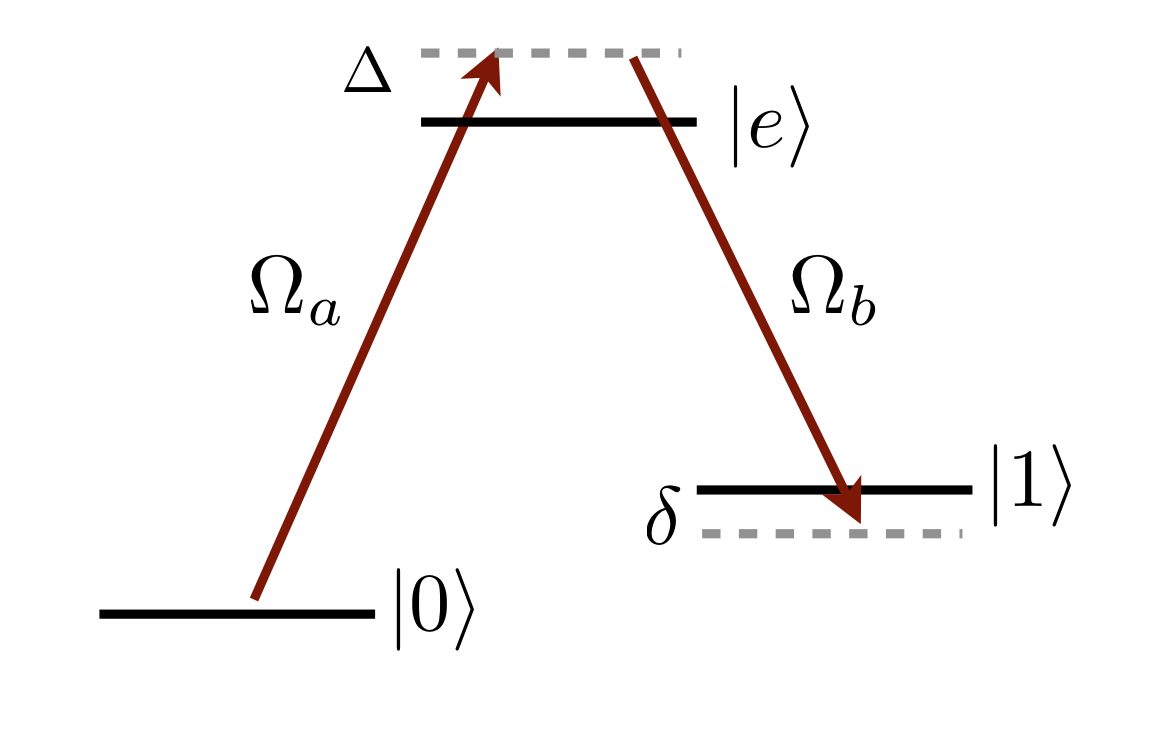
49bc3fd69abc4dd2afe8f7eb58233e4f

We consider here the case of two-photon ground-state Raman transitions from \(\vert 0 \rangle = \vert f_0,m_{f_0}\rangle\) to \(\vert 1 \rangle = \vert f_1,m_{f_1}\rangle\) via an intermediate excited state \(\vert e\rangle = \vert f_e,m_{f_e}\rangle\). In the rotating wave approximation, the Hamiltonian can be written as

\begin{equation} \mathcal{H} = \hbar\begin{pmatrix} 0 & \Omega^a_{0\rightarrow f_e}/2 & 0 \\\Omega^a_{0\rightarrow f_e}/2 & -\Delta & \Omega^b_{1\rightarrow f_e}/2 \\ 0 & \Omega^b_{1\rightarrow f_e}/2 & -\delta\end{pmatrix}, \end{equation}

where \(\Omega^a_{0\rightarrow f_e}\) is the Rabi frequency from \(\vert 0\rangle\rightarrow\vert e\rangle\) due to laser A and \(\Omega^b_{1\rightarrow f_e}\) is the Rabi frequency from \(\vert 1\rangle\rightarrow\vert e\rangle\) due to laser B, \(\Delta=(\Delta_a+\Delta_a)/2\) is the average detuning from the intermediate state and \(\delta=\Delta_a-\Delta_b\) is the two-photon detuning.

In the limit \(\Delta \gg \Omega^a,\Omega^b,\Gamma_e\) the intermediate excited state can be adiabatically elliminiated leading to an effective two-photon Rabi frequency \(\Omega_R = \Omega^a\Omega^b/2\Delta\) and an effective detuning \(\delta_\mathrm{eff}=\delta+\Delta_\mathrm{AC}\) where \(\Delta_\mathrm{AC}\) is the differential Stark shift given by

\begin{equation} \Delta_\mathrm{AC} = \frac{\vert\Omega^b_{0\rightarrow f_e}\vert^2}{4\Delta} - \frac{\vert\Omega^a_{1\rightarrow f_e}\vert^2}{4\Delta}. \end{equation}

On the two-photon transition (\(\delta_\mathrm{eff}=0\)), the probability of spontanteous emission during a \(\pi\)-pulse can be evaluated from \(P_\mathrm{sc}=\Gamma_e\rho_e\tau_\pi\), where \(\tau_\pi=\pi/\Omega_R\) is the \(\pi\)-pulse duration and \(\rho_e\) is the excited state population given by

\begin{equation} \rho_e = \frac{1}{2}\left(\frac{\vert\Omega^a_{0\rightarrow f_e}\vert^2}{2\Delta^2}+\frac{\vert\Omega^b_{1\rightarrow f_e}\vert^2}{2\Delta^2}\right). \end{equation}

For a multi-level atom, the terms describing Raman transition, diffrential AC Stark shift and scattering probability must be calculated by summing over the \(\vert f_e,m_{f_e}\rangle\) states of the intermediate excited state. Additionally, for transitions between hyperfine ground states separated by frequency \(\omega_{01}\) we must also account for the off-resonant AC Stark shift and scattering terms arising from laser A acting on \(\vert 1 \rangle\) with detuning \(\Delta'=\Delta+\omega_{01}\) and laser B acting on \(\vert 0 \rangle\) with detuning \(\Delta'=\Delta-\omega_{01}\).

\begin{align} \Omega_R&=\displaystyle\sum_{f_e,m_{f_e}}\frac{\Omega^a_{0\rightarrow f_e}\Omega^b_{1\rightarrow f_e}}{2(\Delta-\Delta_{f_e})}\\ \Delta_{\mathrm{AC}} &= \displaystyle\sum_{f_e,m_{f_e}}\left[\frac{\vert\Omega^a_{0\rightarrow f_e}\vert^2-\vert\Omega^b_{1\rightarrow f_e}\vert^2}{4(\Delta-\Delta_{f_e})}+\frac{\vert\Omega^a_{1\rightarrow f_e}\vert^2}{4(\Delta+\omega_{01}-\Delta_{f_e})}-\frac{\vert\Omega^b_{0\rightarrow f_e}\vert^2}{4(\Delta-\omega_{01}-\Delta_{f_e})}\right],\\ P_\mathrm{sc} &= \frac{\Gamma_et_\pi}{2}\displaystyle\sum_{f_e,m_{f_e}}\left[\frac{\vert\Omega^a_{0\rightarrow f_e}\vert^2}{2(\Delta-\Delta_{f_e})^2}+\frac{\vert\Omega^b_{1\rightarrow f_e}\vert^2}{2(\Delta-\Delta_{f_e})^2}+\frac{\vert\Omega^a_{1\rightarrow f_e}\vert^2}{4(\Delta+\omega_{01}-\Delta_{f_e})^2}+\frac{\vert\Omega^b_{0\rightarrow f_e}\vert^2}{4(\Delta-\omega_{01}-\Delta_{f_e})^2}\right], \end{align}

OmegaR, AC, Psc = groundStateRamanTransition(Pa, wa, qa, Pb, wb, qb, Delta, f0, mf0, f1, mf1, ne, le, je)

Returns two-photon Rabi frequency \(\Omega_R\), differential AC Starkshift \(\Delta_\mathrm{AC}\) and scattering probability \(P_\mathrm{sc}\) for transition from \(\vert f_0,m_{f_0}\rangle\rightarrow\vert f_1,m_{f_1}\rangle\) via intermediate excited state with quantum numbers \(n_e,\ell_e,j_e\) with detuning \(\Delta\) from excited state centre of mass using laser \(a/b\) with power \(P\), waist \(w\) and polarisation \(q\) driving transitions from \(f_0,f_1\) respectively.

[4]:

# Test Raman Transition Calculation
# ==================================

# Laser Parameters
Pa = 0.1e-3
wa = 5e-6
qa = -1
Pb = 0.1e-3
wb = 5e-6
qb = -1

# Detuning Array
Delta0 = -50e9 * 2 * np.pi
Delta = np.linspace(-150, 150, 10000) * 1e9 * 2 * np.pi

# D1 Line
ne = 6
le = 1
je = 0.5
f1 = 4
mf1 = 0
f0 = 3
mf0 = 0
OmR, AC, Psc = cs.groundStateRamanTransition(
    Pa, wa, qa, Pb, wb, qb, Delta0, f0, mf0, f1, mf1, ne, le, je
)
print(
    "\nRaman Transitions |%d,%d> to |%d,%d> via %dP_%d/2"
    % (f1, mf1, f0, mf0, ne, je * 2)
)
print(
    "\tParameters:\tDelta/2pi = %2.f GHz, Pa = %1.2f mW, wa = %2.1f um, Pa = %1.2f mW, wa = %2.1f um"
    % (Delta0 / 2.0 / np.pi * 1e-9, Pa * 1e3, wa * 1e6, Pb * 1e3, wb * 1e6)
)
print(
    "\tResults:\tOmR/2pi = %2.5f MHz, AC/2pi = %2.5f MHz, Psc = %f"
    % (OmR / 2.0 / np.pi * 1e-6, AC / 2.0 / np.pi * 1e-6, Psc)
)

# D2 Line
ne = 6
le = 1
je = 1.5
OmR, AC, Psc = cs.groundStateRamanTransition(
    Pa, wa, qa, Pb, wb, qb, Delta0, f0, mf0, f1, mf1, ne, le, je
)
print(
    "\nRaman Transitions |%d,%d> to |%d,%d> via %dP_%d/2"
    % (f1, mf1, f0, mf0, ne, je * 2)
)
print(
    "\tParameters:\tDelta/2pi = %2.f GHz, Pa = %1.2f mW, wa = %2.1f um, Pa = %1.2f mW, wa = %2.1f um"
    % (Delta0 / 2.0 / np.pi * 1e-9, Pa * 1e3, wa * 1e6, Pb * 1e3, wb * 1e6)
)
print(
    "\tResults:\tOmR/2pi = %2.5f MHz, AC/2pi = %2.5f MHz, Psc = %f"
    % (OmR / 2.0 / np.pi * 1e-6, AC / 2.0 / np.pi * 1e-6, Psc)
)

# 7P1/2
ne = 7
le = 1
je = 0.5
Pa = 10e-3
Pb = 10e-3
OmR, AC, Psc = cs.groundStateRamanTransition(
    Pa, wa, qa, Pb, wb, qb, Delta0, f0, mf0, f1, mf1, ne, le, je
)
print(
    "\nRaman Transitions |%d,%d> to |%d,%d> via %dP_%d/2"
    % (f1, mf1, f0, mf0, ne, je * 2)
)
print(
    "\tParameters:\tDelta/2pi = %2.f GHz, Pa = %1.2f mW, wa = %2.1f um, Pa = %1.2f mW, wa = %2.1f um"
    % (Delta0 / 2.0 / np.pi * 1e-9, Pa * 1e3, wa * 1e6, Pb * 1e3, wb * 1e6)
)
print(
    "\tResults:\tOmR/2pi = %2.5f MHz, AC/2pi = %2.5f MHz, Psc = %f"
    % (OmR / 2.0 / np.pi * 1e-6, AC / 2.0 / np.pi * 1e-6, Psc)
)

# 7P3/2
ne = 7
le = 1
je = 1.5
Pa = 10e-3
Pb = 10e-3
OmR, AC, Psc = cs.groundStateRamanTransition(
    Pa, wa, qa, Pb, wb, qb, Delta0, f0, mf0, f1, mf1, ne, le, je
)
print(
    "\nRaman Transitions |%d,%d> to |%d,%d> via %dP_%d/2"
    % (f1, mf1, f0, mf0, ne, je * 2)
)
print(
    "\tParameters:\tDelta/2pi = %2.f GHz, Pa = %1.2f mW, wa = %2.1f um, Pa = %1.2f mW, wa = %2.1f um"
    % (Delta0 / 2.0 / np.pi * 1e-9, Pa * 1e3, wa * 1e6, Pb * 1e3, wb * 1e6)
)
print(
    "\tResults:\tOmR/2pi = %2.5f MHz, AC/2pi = %2.5f MHz, Psc = %f"
    % (OmR / 2.0 / np.pi * 1e-6, AC / 2.0 / np.pi * 1e-6, Psc)
)

# Prepare Output Figure
f, ax = plt.subplots(1, 3, figsize=(12, 5))
ax[0].set_xlabel(r"$\Delta/2\pi$ (GHz)")
ax[0].set_ylabel(r"$\Omega/2\pi$ (MHz)")
ax[0].set_ylim([-20, 20])
ax[1].set_xlabel(r"$\Delta/2\pi$ (GHz)")
ax[1].set_ylabel(r"$\Delta_\mathrm{AC}/2\pi$ (MHz)")
ax[1].set_ylim([-20, 20])
ax[2].set_xlabel(r"$\Delta/2\pi$ (GHz)")
ax[2].set_ylabel(r"$P_\mathrm{sc}$")
ax[2].set_ylim([0, 0.01])

# Reset to D2 Line
ne = 6
le = 1
je = 1.5
f1 = 4
mf1 = 0
f0 = 3
mf0 = 0
Pa = 0.1e-3
wa = 5e-6
qa = -1
Pb = 0.1e-3
wb = 5e-6
qb = -1

for mf in range(-3, 4):
    OmR, AC, Psc = cs.groundStateRamanTransition(
        Pa, wa, qa, Pb, wb, qb, Delta, f1, mf, f0, mf + qa - qb, ne, le, je
    )
    ax[0].plot(Delta / (2e9 * np.pi), OmR / (2e6 * np.pi))
    ax[1].plot(Delta / (2e9 * np.pi), AC / (2e6 * np.pi))
    ax[2].plot(
        Delta / (2e9 * np.pi),
        Psc,
        label=format(
            "$\\vert%d,%d\\rangle\\rightarrow\\vert%d,%d\\rangle$"
            % (f1, mf, f0, mf)
        ),
    )
ax[2].legend(loc=4)
ax[1].set_title("D2 Raman Transitions")
plt.show()


Raman Transitions |4,0> to |3,0> via 6P_1/2
        Parameters:     Delta/2pi = -50 GHz, Pa = 0.10 mW, wa = 5.0 um, Pa = 0.10 mW, wa = 5.0 um
        Results:        OmR/2pi = -10.58926 MHz, AC/2pi = 2.01241 MHz, Psc = 0.000603

Raman Transitions |4,0> to |3,0> via 6P_3/2
        Parameters:     Delta/2pi = -50 GHz, Pa = 0.10 mW, wa = 5.0 um, Pa = 0.10 mW, wa = 5.0 um
        Results:        OmR/2pi = 10.51457 MHz, AC/2pi = 3.86727 MHz, Psc = 0.001380

Raman Transitions |4,0> to |3,0> via 7P_1/2
        Parameters:     Delta/2pi = -50 GHz, Pa = 10.00 mW, wa = 5.0 um, Pa = 10.00 mW, wa = 5.0 um
        Results:        OmR/2pi = -3.97773 MHz, AC/2pi = 0.75654 MHz, Psc = 0.000136

Raman Transitions |4,0> to |3,0> via 7P_3/2
        Parameters:     Delta/2pi = -50 GHz, Pa = 10.00 mW, wa = 5.0 um, Pa = 10.00 mW, wa = 5.0 um
        Results:        OmR/2pi = 8.98075 MHz, AC/2pi = 3.37987 MHz, Psc = 0.000325

Two-photon Rydberg excitation#

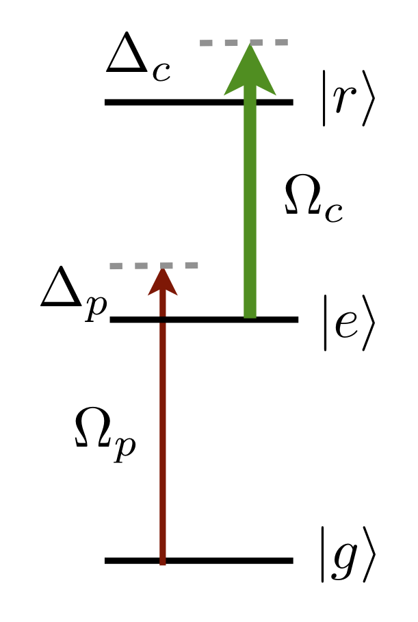
8fc0b11cd61c4fb095f9e144f6dfdafb

We consider here the case of two-photon ground-state Raman transitions from \(\vert g \rangle = \vert f_g,m_{f_g}\rangle\) to \(\vert r \rangle = \vert n_r,l_r,j_r,m_{j_r}\rangle\) via an intermediate excited state \(\vert e\rangle = \vert f_e,m_{f_e}\rangle\). In the rotating wave approximation, the Hamiltonian can be written as

\begin{equation} \mathcal{H} = \hbar\begin{pmatrix} 0 & \Omega_p/2 & 0 \\\Omega_p/2 & -\Delta_p & \Omega_c/2 \\ 0 & \Omega_c/2 & -\delta\end{pmatrix}, \end{equation}

where \(\Omega_p\) is the Rabi frequency from \(\vert 0\rangle\rightarrow\vert e\rangle\) due to the probe laser and \(\Omega_c\) is the Rabi frequency from \(\vert e\rangle\rightarrow\vert r\rangle\) due to the coupling laser, \(\delta=(\Delta_p+\Delta_c)\) is the two-photon detuning.

In the limit \(\Delta_p \gg \Omega_p,\Omega_c,\Gamma_e\) the intermediate excited state can be adiabatically elliminiated leading to an effective two-photon Rabi frequency \(\Omega_R = \Omega_p\Omega_c/2\Delta\) and an effective detuning \(\delta_\mathrm{eff}=\delta+\Delta_\mathrm{AC}\) where \(\Delta_\mathrm{AC}\) is the differential Stark shift given by

\begin{equation} \Delta_\mathrm{AC} = \frac{\vert\Omega_p\vert^2}{4\Delta_p} - \frac{\vert\Omega_c\vert^2}{4\Delta_c}. \end{equation}

\begin{equation} \rho_e = \frac{1}{2}\left(\frac{\vert\Omega_p\vert^2}{2\Delta_p^2}+\frac{\vert\Omega_c\vert^2}{2\Delta_c^2}\right). \end{equation}

\begin{align} \Omega_R&=\displaystyle\sum_{f_e,m_{f_e}}\frac{\Omega_p^{g\rightarrow f_e}\Omega_c^{f_e\rightarrow r}}{2(\Delta-\Delta_{f_e})}\\ \Delta_{\mathrm{AC}_g} &= \displaystyle\sum_{f_e,m_{f_e}}\frac{\vert\Omega_p^{g\rightarrow f_e}\vert^2}{4(\Delta-\Delta_{f_e})}\\ \Delta_{\mathrm{AC}_r} &= \displaystyle\sum_{f_e,m_{f_e}}\frac{\vert\Omega_c^{f_e\rightarrow r}\vert^2}{4(\Delta-\Delta_{f_e})}\\ P_\mathrm{sc} &= \frac{\Gamma_et_\pi}{2}\displaystyle\sum_{f_e,m_{f_e}}\left[\frac{\vert\Omega_p^{g\rightarrow f_e}\vert^2}{2(\Delta-\Delta_{f_e})^2}+\frac{\vert\Omega_c^{f_e\rightarrow r}\vert^2}{2(\Delta-\Delta_{f_e})^2}\right] \end{align}

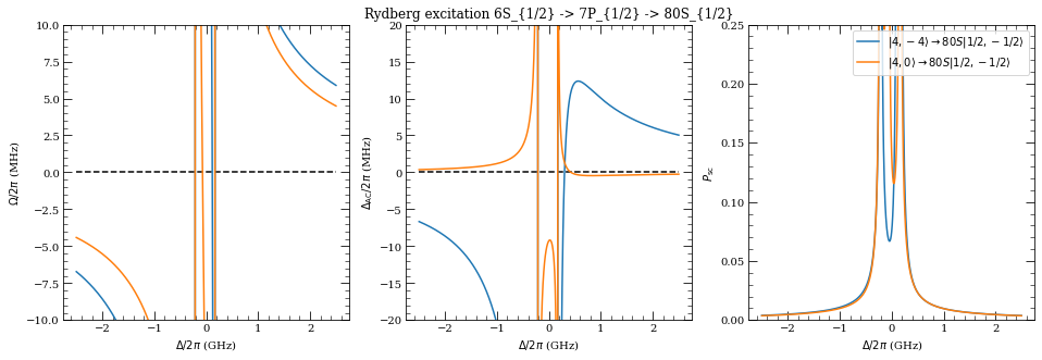
OmegaR, ACg, ACr, Psc = twoPhotonRydbergExcitation(Pp, wp, qp, Pc, wc, qc, Delta, fg, mfg, ne, le, je, nr, lr, jr, mjr)

Returns two-photon Rabi frequency \(\Omega_R\), ground-state AC Starkshift \(\Delta_\mathrm{AC_g}\), Rydberg-state AC Starkshift \(\Delta_\mathrm{AC_r}\) and scattering probability \(P_\mathrm{sc}\) for transition from \(\vert f_g,m_{f_g}\rangle\rightarrow n_rL_{j_r}\vert j_r,m_{j_r}\rangle\) via intermediate excited state with quantum numbers \(n_e,\ell_e,j_e\) with detuning \(\Delta\) from excited state centre of mass driven by probe/coupling lasers with power \(P\), waist \(w\) and polarisation \(q\) driving transitions from \(\vert g\rangle,\vert r\rangle\) respectively.

[5]:

# Rydberg Excitation vs 6P3/2
Pp = 500e-9
wp = 3e-6
qp = 1
Pc = 200e-3
wc = 5e-6
qc = -1
# Ground State
fg = 4
mfg = 0
# Excited state (6P3/2)
ne = 6
le = 1
je = 1.5
# Rydberg state (82S1/2)
nr = 80
lr = 0
jr = 0.5
mjr = -0.5

SPD = "SPD"

# Detuning Array
Delta0 = 1.1e9 * 2 * np.pi
Delta = np.linspace(-2.5, 2.5, 1001) * 1e9 * 2 * np.pi

[OmR, ACg, ACr, Psc] = cs.twoPhotonRydbergExcitation(
    Pp, wp, qp, Pc, wc, qc, Delta0, fg, mfg, ne, le, je, nr, lr, jr, mjr
)
print(
    "\nRydberg Excitation 6S1/2 |%d,%d> to %d%c |%d/2,%d/2> via %dP_%d/2"
    % (fg, mfg, nr, SPD[lr], 2 * jr, 2 * mjr, ne, je * 2)
)
print(
    "\n\tParameters:\tDelta/2pi = %2.2f GHz, Pp = %1.2f uW, wp = %2.1f um, qp=%d, Pc = %1.2f mW, wc = %2.1f um, qc=%d"
    % (
        Delta0 / 2.0 / np.pi * 1e-9,
        Pp * 1e6,
        wp * 1e6,
        qp,
        Pc * 1e3,
        wc * 1e6,
        qc,
    )
)
print(
    "\n\tResults:\tOmR/2pi = %2.5f MHz\n\t\t\tACg/2pi = %2.5f MHz\n\t\t\tACr/2pi = %2.5f MHz\n\t\t\tDelta_AC/2pi = %2.5f MHz\n\t\t\tPsc = %f"
    % (
        OmR / 2.0 / np.pi * 1e-6,
        ACg / 2.0 / np.pi * 1e-6,
        ACr / 2.0 / np.pi * 1e-6,
        (ACg - ACr) / 2.0 / np.pi * 1e-6,
        Psc,
    )
)

# Prepare Output Figure
[f, ax] = plt.subplots(1, 3, figsize=(16, 5))
ax[0].set_xlabel(r"$\Delta/2\pi$ (GHz)")
ax[0].set_ylabel(r"$\Omega/2\pi$ (MHz)")
ax[0].set_ylim([-10, 10])
ax[1].set_xlabel(r"$\Delta/2\pi$ (GHz)")
ax[1].set_ylabel(r"$\Delta_\mathrm{AC}/2\pi$ (MHz)")
ax[1].set_ylim([-20, 20])
ax[2].set_xlabel(r"$\Delta/2\pi$ (GHz)")
ax[2].set_ylabel(r"$P_\mathrm{sc}$")
ax[2].set_ylim([0, 0.25])
ax[0].plot(Delta / (2e9 * np.pi), 0 * Delta, "k--")
ax[1].plot(Delta / (2e9 * np.pi), 0 * Delta, "k--")

mj = -jr - 1
for m in range(int(2 * jr + 1)):
    mj += 1
    for mfg in [-fg, 0, fg]:
        [OmR, ACg, ACr, Psc] = cs.twoPhotonRydbergExcitation(
            Pp, wp, qp, Pc, wc, qc, Delta, fg, mfg, ne, le, je, nr, lr, jr, mj
        )
        if np.sum(np.abs(OmR)) > 0.1:
            ax[0].plot(Delta / (2e9 * np.pi), OmR / (2e6 * np.pi))
            ax[1].plot(Delta / (2e9 * np.pi), (ACg - ACr) / (2e6 * np.pi))
            ax[2].plot(
                Delta / (2e9 * np.pi),
                Psc,
                label=format(
                    "$\\vert%d,%d\\rangle\\rightarrow%d%c\\vert%1.0f/2,%1.0f/2\\rangle$"
                    % (fg, mfg, nr, SPD[lr], 2 * jr, 2 * mj)
                ),
            )
ax[2].legend(loc=1)
ax[1].set_title(
    "Rydberg excitation 6S_{1/2} -> %dP_{%1.f/2} -> %d%c_{%1.0f/2}"
    % (ne, 2 * je, nr, SPD[lr], 2 * jr)
)


plt.show()


Rydberg Excitation 6S1/2 |4,0> to 80S |1/2,-1/2> via 6P_3/2

        Parameters:     Delta/2pi = 1.10 GHz, Pp = 0.50 uW, wp = 3.0 um, qp=1, Pc = 200.00 mW, wc = 5.0 um, qc=-1

        Results:        OmR/2pi = -3.31688 MHz
                        ACg/2pi = 7.64903 MHz
                        ACr/2pi = 7.54096 MHz
                        Delta_AC/2pi = 0.10807 MHz
                        Psc = 0.077362

/home/nikola/Documents/Desktop/github/newARC3/ARC-Alkali-Rydberg-Calculator/doc/../arc/alkali_atom_functions.py:2616: RuntimeWarning: divide by zero encountered in true_divide
  tau_pi = pi / abs(OmegaR)

[6]:

# Rydberg Excitation vs 7P1/2
Pp = 1.535e-3
wp = 5e-6
qp = 1
Pc = 20e-3
wc = 3e-6
qc = -1
# Ground State
fg = 4
mfg = 0
# Excited state (7P1/2)
ne = 7
le = 1
je = 0.5
# Rydberg state (82S1/2)
nr = 80
lr = 0
jr = 0.5
mjr = -0.5

# Detuning Array
Delta0 = 1e9 * 2 * np.pi
Delta = np.linspace(-2.5, 2.5, 1001) * 1e9 * 2 * np.pi

[OmR, ACg, ACr, Psc] = cs.twoPhotonRydbergExcitation(
    Pp, wp, qp, Pc, wc, qc, Delta0, fg, mfg, ne, le, je, nr, lr, jr, mjr
)
print(
    "\nRydberg Excitation 6S1/2 |%d,%d> to %d%c |%d/2,%d/2> via %dP_%d/2"
    % (fg, mfg, nr, SPD[lr], 2 * jr, 2 * mjr, ne, je * 2)
)
print(
    "\n\tParameters:\tDelta/2pi = %2.2f GHz, Pp = %1.2f uW, wp = %2.1f um, qp=%d, Pc = %1.2f mW, wc = %2.1f um, qc=%d"
    % (
        Delta0 / 2.0 / np.pi * 1e-9,
        Pp * 1e6,
        wp * 1e6,
        qp,
        Pc * 1e3,
        wc * 1e6,
        qc,
    )
)
print(
    "\n\tResults:\tOmR/2pi = %2.5f MHz\n\t\t\tACg/2pi = %2.5f MHz\n\t\t\tACr/2pi = %2.5f MHz\n\t\t\tDelta_AC/2pi = %2.5f MHz\n\t\t\tPsc = %f"
    % (
        OmR / 2.0 / np.pi * 1e-6,
        ACg / 2.0 / np.pi * 1e-6,
        ACr / 2.0 / np.pi * 1e-6,
        (ACg - ACr) / 2.0 / np.pi * 1e-6,
        Psc,
    )
)

# Prepare Output Figure
[f, ax] = plt.subplots(1, 3, figsize=(16, 5))
ax[0].set_xlabel(r"$\Delta/2\pi$ (GHz)")
ax[0].set_ylabel(r"$\Omega/2\pi$ (MHz)")
ax[0].set_ylim([-10, 10])
ax[1].set_xlabel(r"$\Delta/2\pi$ (GHz)")
ax[1].set_ylabel(r"$\Delta_\mathrm{AC}/2\pi$ (MHz)")
ax[1].set_ylim([-20, 20])
ax[2].set_xlabel(r"$\Delta/2\pi$ (GHz)")
ax[2].set_ylabel(r"$P_\mathrm{sc}$")
ax[2].set_ylim([0, 0.25])
ax[0].plot(Delta / (2e9 * np.pi), 0 * Delta, "k--")
ax[1].plot(Delta / (2e9 * np.pi), 0 * Delta, "k--")

SPD = "SPD"

mj = -jr - 1
for m in range(int(2 * jr + 1)):
    mj += 1
    for mfg in [-fg, 0, fg]:
        [OmR, ACg, ACr, Psc] = cs.twoPhotonRydbergExcitation(
            Pp, wp, qp, Pc, wc, qc, Delta, fg, mfg, ne, le, je, nr, lr, jr, mj
        )
        if np.sum(np.abs(OmR)) > 0.1:
            ax[0].plot(Delta / (2e9 * np.pi), OmR / (2e6 * np.pi))
            ax[1].plot(Delta / (2e9 * np.pi), (ACg - ACr) / (2e6 * np.pi))
            ax[2].plot(
                Delta / (2e9 * np.pi),
                Psc,
                label=format(
                    "$\\vert%d,%d\\rangle\\rightarrow%d%c\\vert%1.0f/2,%1.0f/2\\rangle$"
                    % (fg, mfg, nr, SPD[lr], 2 * jr, 2 * mj)
                ),
            )
ax[2].legend(loc=1)
ax[1].set_title(
    "Rydberg excitation 6S_{1/2} -> %dP_{%1.f/2} -> %d%c_{%1.0f/2}"
    % (ne, 2 * je, nr, SPD[lr], 2 * jr)
)


plt.show()


Rydberg Excitation 6S1/2 |4,0> to 80S |1/2,-1/2> via 7P_1/2

        Parameters:     Delta/2pi = 1.00 GHz, Pp = 1535.00 uW, wp = 5.0 um, qp=1, Pc = 20.00 mW, wc = 3.0 um, qc=-1

        Results:        OmR/2pi = 11.70666 MHz
                        ACg/2pi = 16.15630 MHz
                        ACr/2pi = 16.59130 MHz
                        Delta_AC/2pi = -0.43500 MHz
                        Psc = 0.009768

/home/nikola/Documents/Desktop/github/newARC3/ARC-Alkali-Rydberg-Calculator/doc/../arc/alkali_atom_functions.py:2616: RuntimeWarning: divide by zero encountered in true_divide
  tau_pi = pi / abs(OmegaR)

Magnetic Functions#

getLandegj(l, j, s=0.5)

Returns fine-structure Landé g-factor \(g_J\)

\begin{equation} g_J\simeq 1+\frac{j(j+1)+s(s+1)-l(l+1)}{2j(j+1)} \end{equation}

getLandegjExact(l, j, s=0.5)

Returns fine-structure Landé g-factor \(g_J\) using precise \(g_L,\) \(g_S\) values

\begin{equation} g_J=g_L\frac{j(j+1)-s(s+1)+l(l+1)}{2j(j+1)}+g_S\frac{j(j+1)+s(s+1)-l(l+1)}{2j(j+1)} \end{equation}

getLandegf(l, j, f, s=0.5)

Returns hyperfine-structure Landé g-factor \(g_F\)

\begin{equation} g_F\simeq g_J\frac{f(f+1)-I(I+1)+j(j+1)}{2f(f+1)} \end{equation}

getLandegfExact(l, j, f, s=0.5)

Returns hyperfine-structure Landé g-factor \(g_F\) using precise \(g_L,\) \(g_S\), \(g_I\) values

\begin{equation} g_F=g_J\frac{f(f+1)-I(I+1)+j(j+1)}{2f(f+1)}+g_I\frac{f(f+1)+I(I+1)-j(j+1)}{2f(f+1)} \end{equation}

Ez = breitRabi(l, j, B, Ahfs, Bhfs)

Return exact Zeman energy levels for the l,j manifold via diagonalisation of \(\mathcal{H}=\mathcal{H}_\mathrm{hfs}+\mathcal{H}_\mathrm{Z}\) where \(\mathcal{H}_\mathrm{hfs}\) is the Hamiltonian for the hyperfine interaction given by \begin{equation} \mathcal{H}_\mathrm{hfs}=A_\mathrm{hfs}I\cdot J + B_\mathrm{hfs}\frac{3(I\cdot J)^2+3/2 I\cdot J -I^2J^2}{2I(2I+1)2J(2J+1)}, \end{equation} and \(\mathcal{H}_Z\) is the Hamiltonian for the Zeeman interaction given by \begin{equation} \mathcal{H}_Z=\frac{\mu_B}{\hbar}(g_J J_z+g_I I_z)B_z \end{equation}

For the \(j=1/2\) ground-state, this can be compared against the breitRabi formula [1]

:nbsphinx-math:`begin{equation}: E_{vert j=1/2,m_j,I,m_Irangle} = -frac{A_mathrm{hfs}(I+1/2)}{2(2I+1)}+g_Imu_B m B_z pm frac{A_mathrm{hfs}(I+1/2)}{2}left(1+frac{4mx}{2I+1}+x^2right)^{1/2},

end{equation}` where \(m=m_I\pm m_j\) and \begin{equation} x=\frac{g_j-g_I)\mu_B B_z}{A_\mathrm{hfs}(I+1/2)}. \end{equation}

[7]:

# Lande g-factors
gj = cs.getLandegj(0, 0.5)
gf3 = cs.getLandegf(0, 0.5, 4)
gf4 = cs.getLandegf(0, 0.5, 4)
print("Cs 6S1/2 gJ = %2.2f, F=3 gF = %2.2f, F=4 gF = %2.2f," % (gj, gf3, gf4))
gj = cs.getLandegjExact(0, 0.5)
gf3 = cs.getLandegfExact(0, 0.5, 4)
gf4 = cs.getLandegfExact(0, 0.5, 4)
print("Cs 6S1/2 gJ = %f, F=3 gF = %f, F=4 gF = %f," % (gj, gf3, gf4))

# Zeeman Interaction 6S1/2
# ========================
# Define State of Interest
lg = 0
jg = 1 / 2

# B-Field (G)
B = np.linspace(0, 5000, 101) * 1e-4
# Exact-Diagonalisation (Breit-Rabi)
en, f, mf = cs.breitRabi(6, lg, jg, B)

f, ax = plt.subplots(3, 1, figsize=(12, 10))
ax[0].plot(B * 1e4, en * 1e-9, "k")
ax[0].set_xlabel(r"$B_z$ (G)")
ax[0].set_ylabel(r"$E$ (GHz)")
ax[0].set_title(r"Breit-Rabi Diagram $6S_{1/2}$")

# Plot Breit-Rabi Formula
# =======================
#   Steck Eq(25)
#                         dEhfs                dEhfs      4mx
#   E(j=1/2,mj;I,mI) = - ------- + gI*uB*m*B ± ----- (1+ ----- + x^2)^{1/2}
#                        2(2I+1)                 2        2I+1
#
#   where m=mI±mj to match sign above and x=(gj-gI)uB*B/dEhfs
uB = physical_constants["Bohr magneton in Hz/T"][0]
Ahfs, Bhfs = cs.getHFSCoefficients(6, 0, 0.5)
qhfs = Ahfs * (cs.I + jg)
gj = cs.getLandegjExact(lg, jg)
# Rescale to x
x = (gj - cs.gI) * uB * B / qhfs

Ebr = np.zeros(np.shape(en))

ctr = -1
for mI in np.arange(-cs.I, 1 + cs.I):
    for mj in np.arange(-jg, 1 + jg):
        m = mI + mj
        ctr += 1
        if abs(m) == (cs.I + jg):
            Ebr[:, ctr] = (
                qhfs * cs.I / (2 * cs.I + 1)
                + np.sign(mj) * 1 / 2 * (gj + 2 * cs.gI) * uB * B
            )
        else:
            Ebr[:, ctr] = (
                -qhfs / (2 * (2 * cs.I + 1))
                + cs.gI * uB * m * B
                + np.sign(mj)
                * qhfs
                / 2
                * np.sqrt(1 + 4 * m * x / (2 * cs.I + 1) + x**2)
            )

ax[0].plot(B * 1e4, Ebr * 1e-9, "r.")

ax[0].text(
    0,
    min(en[0, :]) * 1.5e-9,
    r"$F=3$",
    horizontalalignment="center",
    fontsize=12,
)
ax[0].text(
    0,
    max(en[0, :]) * 1.2e-9,
    r"$F=4$",
    horizontalalignment="center",
    fontsize=12,
)


# 6P1/2

# Exact-Diagonalisation (Breit-Rabi)
B = np.linspace(0, 2000, 101) * 1e-4
en, f, mf = cs.breitRabi(6, 1, 0.5, B)
ax[1].plot(B * 1e4, en * 1e-9, "k")
ax[1].set_xlabel(r"$B_z$ (G)")
ax[1].set_ylabel(r"$E$ (GHz)")
ax[1].set_title(r"Breit-Rabi Diagram $6P_{1/2}$")
ax[1].text(
    0,
    min(en[0, :]) * 1.5e-9,
    r"$F=3$",
    horizontalalignment="center",
    fontsize=12,
)
ax[1].text(
    0,
    max(en[0, :]) * 1.2e-9,
    r"$F=4$",
    horizontalalignment="center",
    fontsize=12,
)

# Exact-Diagonalisation (Breit-Rabi)
B = np.linspace(0, 500, 101) * 1e-4
en, f, mf = cs.breitRabi(6, 1, 1.5, B)
ax[2].plot(B * 1e4, en * 1e-9, "k")
ax[2].set_xlabel(r"$B_z$ (G)")
ax[2].set_ylabel(r"$E$ (GHz)")
ax[2].set_title(r"Breit-Rabi Diagram $6P_{3/2}$")
ax[2].text(
    0, min(en[0, :]) * 2e-9, r"$F=2$", horizontalalignment="center", fontsize=12
)
ax[2].text(
    0,
    max(en[0, :]) * 1.7e-9,
    r"$F=5$",
    horizontalalignment="center",
    fontsize=12,
)

plt.show()

Cs 6S1/2 gJ = 2.00, F=3 gF = 0.25, F=4 gF = 0.25,
Cs 6S1/2 gJ = 2.002319, F=3 gF = 0.249941, F=4 gF = 0.249941,

[ ]: