Divalent atom functions

Note

This is a completely new module added in ARC 3.0.0 version. See more at E. J. Robertson, N. Šibalić, R. M. Potvliege and M. P. A. Jones, *Computer Physics Communications* **261**, 107814 (2021) `https://doi.org/10.1016/j.cpc.2020.107814 .

Overview

DivalentAtom Methods

DivalentAtom.getDipoleMatrixElement(n1, l1, ...)	Dipole matrix element \(\langle n_1 l_1 j_1 m_{j_1} |e\mathbf{r}|\ n_2 l_2 j_2 m_{j_2}\rangle\) in units of \(a_0 e\)
DivalentAtom.getTransitionWavelength(n1, l1, ...)	Calculated transition wavelength (in vacuum) in m.
DivalentAtom.getTransitionFrequency(n1, l1, ...)	Calculated transition frequency in Hz
DivalentAtom.getRabiFrequency(n1, l1, j1, ...)	Returns a Rabi frequency for resonantly driven atom in a center of TEM00 mode of a driving field
DivalentAtom.getRabiFrequency2(n1, l1, j1, ...)	Returns a Rabi frequency for resonant excitation with a given electric field amplitude
DivalentAtom.getStateLifetime(n, l, j[, ...])	Returns the lifetime of the state (in s)
DivalentAtom.getTransitionRate(n1, l1, j1, ...)	Transition rate due to coupling to vacuum modes (black body included)
DivalentAtom.getReducedMatrixElementJ_asymmetric(n1, ...)	Reduced matrix element in \(J\) basis, defined in asymmetric notation.
DivalentAtom.getReducedMatrixElementJ(n1, ...)	Reduced matrix element in \(J\) basis (symmetric notation)
DivalentAtom.getReducedMatrixElementL(n1, ...)	Reduced matrix element in \(L\) basis (symmetric notation)
DivalentAtom.getRadialMatrixElement(n1, l1, ...)	Radial part of the dipole matrix element
DivalentAtom.getQuadrupoleMatrixElement(n1, ...)	Radial part of the quadrupole matrix element
DivalentAtom.getPressure(temperature)	Vapour pressure (in Pa) at given temperature
DivalentAtom.getNumberDensity(temperature)	Atom number density at given temperature
DivalentAtom.getAverageInteratomicSpacing(...)	Returns average interatomic spacing in atomic vapour
DivalentAtom.getEnergy(n, l, j[, s])	Energy of the level relative to the ionisation level (in eV)
DivalentAtom.getZeemanEnergyShift(l, j, mj, ...)	Retuns linear (paramagnetic) Zeeman shift.
DivalentAtom.getQuantumDefect(n, l, j[, s])	Quantum defect of the level.
DivalentAtom.getC6term(n, l, j, n1, l1, j1, ...)	C6 interaction term for the given two pair-states
DivalentAtom.getC3term(n, l, j, n1, l1, j1, ...)	C3 interaction term for the given two pair-states
DivalentAtom.getEnergyDefect(n, l, j, n1, ...)	Energy defect for the given two pair-states (one of the state has two atoms in the same state)
DivalentAtom.getEnergyDefect2(n, l, j, nn, ...)	Energy defect for the given two pair-states
DivalentAtom.updateDipoleMatrixElementsFile()	Updates the file with pre-calculated dipole matrix elements.
DivalentAtom.getRadialCoupling(n, l, j, n1, ...)	Returns radial part of the coupling between two states (dipole and quadrupole interactions only)
DivalentAtom.getAverageSpeed(temperature)	Average (mean) speed at a given temperature
DivalentAtom.getLiteratureDME(n1, l1, j1, ...)	Returns literature information on requested transition.

Detailed documentation

class DivalentAtom(preferQuantumDefects=True, cpp_numerov=True)

Bases: AlkaliAtom

Implements general calculations for Alkaline Earths, and other divalent atoms.

This class inherits arc.alkali_atom_functions.AlkaliAtom . Most of the methods can be directly used from there, and the source for them is provided in the base class. Few methods that are implemented differently for Alkaline Earths are defined here.

Parameters:

• preferQuantumDefects (bool) – Use quantum defects for energy level calculations. If False, uses NIST ASD values where available. If True, uses quantum defects for energy calculations for principal quantum numbers within the range specified in defectFittingRange which is specified for each element and series separately. For principal quantum numbers below this value, NIST ASD values are used if existing, since quantum defects. Default is True.

• cpp_numerov (bool) – This switch for Alkaline Earths at the moment doesn’t have any effect since wavefunction calculation function is not implemented (d.m.e. and quadrupole matrix elements are calculated directly semiclassically)

I: float = 0.0

Nuclear spin

Z: int = 0

Atomic number

a1: List[float] = [0]

Model potential parameters fitted from experimental observations for different l (electron angular momentum)

abundance: float = 1.0

relative isotope abundance

alphaC: float = 0.0

Core polarizability

alpha_d_eff: float = 0

ion core dipole polarisability

alpha_q_eff: float = 0

ion core quadrupole polarisability

breitRabi(n: int, l: int, j: float, B: ndarray[Any, dtype[_ScalarType_co]]) → Tuple[ndarray[Any, dtype[_ScalarType_co]], ndarray[Any, dtype[_ScalarType_co]], ndarray[Any, dtype[_ScalarType_co]]]

Returns exact Zeeman energies math:E_z for states \(\vert F,m_f\rangle\) in the \(\ell,j\) manifold via exact diagonalisation of the Zeeman interaction \(\mathcal{H}_z\) and the hyperfine interaction \(\mathcal{H}_\mathrm{hfs}\) given by equations

\(\mathcal{H}_Z=\frac{\mu_B}{\hbar}(g_J J_z+g_I I_z)B_z\)

and

\(\mathcal{H}_\mathrm{hfs}=A_\mathrm{hfs}I\cdot J + B_\mathrm{hfs}\frac{3(I\cdot J)^2+3/2 I\cdot J -I^2J^2}{2I(2I-1)2J(2J-1)}\).

Parameters:

• n – principal,orbital, total orbital quantum numbers

• l – principal,orbital, total orbital quantum numbers

• j – principal,orbital, total orbital quantum numbers

• B – Magnetic Field (units T)

Returns:

State energy \(E_z\) in SI units (Hz), state f, state mf

Return type:

float

corePotential(l, r)

Not implemented for Alkaline earths

cpp_numerov: bool = True

swich - should the wavefunction be calculated with Numerov algorithm implemented in C++

defectFittingRange: dict = {}

Used for AlkalineEarths to define minimum and maximum principal quantum number for which quantum defects are valid. Ranges are stored under keys defined as state terms ({‘stateLabel’:[minN, maxN]}, e.g. ‘1S0’). Dictionary returns array stating minimal and maximal principal quantum number for which quantum defects were fitted. For example:

limits = self.defectFittingRange['1S0']
print("Minimal n = %d" % limits[0])
print("Maximal n = %d" % limits[1]) 1

dipoleMatrixElementFile: str = ''

location of hard-disk stored dipole matrix elements

effectiveCharge(l, r)

Not implemented for Alkaline earths

elementName: str = 'elementName'

Human-readable element name

energyLevelsExtrapolated = False

flag that is turned to True if the energy levels of this atom were calculated by extrapolating with quantum defects values outside the quantum defect fitting range.

extraLevels: List[Tuple[int, int, int, int]] = []

levels that are for smaller principal quantum number (n) than ground level, but are above in energy due to angular part

gI: float = 0.0

Nuclear g-factor

gL: float = 1.0

Electron Orbital g-factor

getAverageInteratomicSpacing(temperature: float) → float

Returns average interatomic spacing in atomic vapour

See calculation of basic properties example snippet.

Parameters:

temperature (float) – temperature (K) of the atomic vapour

Returns:

average interatomic spacing in m

Return type:

float

getAverageSpeed(temperature: float) → float

Average (mean) speed at a given temperature

Parameters:

temperature (float) – temperature (K)

Returns:

mean speed (m/s)

Return type:

float

getBBRshift(n: int, l: int, j: float, includeLevelsUpTo: int = 0, temperature: float = 0.0, s: float = 0.5) → float

Frequency shift of an atomic state induced by black-body radiation using the Farley-Wing function. Uses getFarleyWing as part of the calculation.

n, l, j (int,int,float): specifies state whose shift we are

calculating

temperatureoptional. Temperature at which the atom

environment is, measured in K. If this parameter is non-zero, user has to specify transitions up to which state (due to black-body decay) should be included in calculation.

includeLevelsUpTo (int): optional and not needed for atom

lifetimes calculated at zero temperature. At non zero temperatures, this specify maximum principal quantum number of the state to which black-body induced transitions will be included. Minimal value of the parameter in that case is \(n+1\)

Returns:

Energy shift in units of frequency (Hz)

Return type:

float

See also

getFarleyWing which is used in calculation.

References: (Farley, John W., and William H. Wing. Physical Review A 23.5 (1981): 2397 doi = {10.1103/PhysRevA.23.2397} )

getBranchingRatio(jg: float, fg: float, mfg: float, je: float, fe: float, mfe: float, s: float = 0.5) → float

Branching ratio for decay from \(\vert j_e,f_e,m_{f_e} \rangle \rightarrow \vert j_g,f_g,m_{f_g}\rangle\)

\(b = \displaystyle\sum_q (2j_e+1)\left(\begin{matrix}f_1 & 1 & f_2 \\-m_{f1} & q & m_{f2}\end{matrix}\right)^2\vert \langle j_e,f_e\vert \vert er \vert\vert j_g,f_g\rangle\vert^2/|\langle j_e || er || j_g \rangle |^2\)

Parameters:

• jg – total orbital, fine basis (total atomic) angular momentum, and projection of total angular momentum for ground state

• fg – total orbital, fine basis (total atomic) angular momentum, and projection of total angular momentum for ground state

• mfg – total orbital, fine basis (total atomic) angular momentum, and projection of total angular momentum for ground state

• je – total orbital, fine basis (total atomic) angular momentum,

• fe – total orbital, fine basis (total atomic) angular momentum,

• mfe – total orbital, fine basis (total atomic) angular momentum,

• state (and projection of total angular momentum for excited)

• s (float) – optional, total spin angular momentum of state. By default 0.5 for Alkali atoms.

Returns:

branching ratio

Return type:

float

getBranchingRatioFStoFS(jg: float, mjg: float, je: float, mje: float, s: float = 0.5) → float

Branching ratio for decay from \(\vert j_e, m_{j_e} \rangle \rightarrow \vert j_g,m_{j_g} \rangle\)

Parameters:

• jg (float) – total orbital angular momentum of the lower energy state

• mjg (float) – projection of the total orbital momentum of the lower energy state

• je (float) – total orbital angular momentum of the higher energy state

• mje (float) – projection of the total orbital angular momentum of the higher energy state

• s (float, optional) – total spin angular momentum of the states. By default 0.5 for Alkali atoms.

Returns:

branching ratio

Return type:

float

getBranchingRatioFStoHFS(jg: float, fg: float, mfg: float, je: float, mje: float, s: float = 0.5) → float

Branching ratio for decay from \(\vert j_e, m_{j_e} \rangle \rightarrow \vert j_g,f_g,m_{f_g} \rangle\)

Parameters:

• jg (float) – total orbital angular momentum of the lower energy state

• fg (float) – hyperfine basis (total atomic) angular momentum of the lower energy state

• mfg (float) – projection of the total angular momentum of the lower energy state

• je (float) – total orbital angular momentum of the higher energy state

• mje (float) – projection of the total orbital angular momentum of the higher energy state

• s (float, optional) – total spin angular momentum of the states. By default 0.5 for Alkali atoms.

Returns:

branching ratio

Return type:

float

getBranchingRatioHFStoFS(jg: float, mjg: float, je: float, fe: float, mfe: float, s: float = 0.5) → float

Branching ratio for decay from \(\vert j_e,f_e,m_{f_e} \rangle \rightarrow \vert j_g,m_{j_g} \rangle\)

Parameters:

• jg (float) – total orbital angular momentum of the lower energy state

• mjg (float) – projection of the total orbital angular momentum of the lower energy state

• je (float) – total orbital angular momentum of the higher energy state

• fe (float) – hyperfine basis (total atomic) angular momentum of the higher energy state

• mfe (float) – projection of the total angular momentum of the higher energy state

• s (float, optional) – total spin angular momentum of the states. By default 0.5 for Alkali atoms.

Returns:

branching ratio

Return type:

float

getC3term(n: int, l: int, j: float, n1: int, l1: int, j1: float, n2: int, l2: int, j2: float, s: float = 0.5) → float

C3 interaction term for the given two pair-states

Calculates \(C_3\) intaraction term for

\(|n,l,j,n,l,j\rangle \leftrightarrow |n_1,l_1,j_1,n_2,l_2,j_2\rangle\)

Parameters:

• n (int) – principal quantum number

• l (int) – orbital angular momentum

• j (float) – total angular momentum

• n1 (int) – principal quantum number

• l1 (int) – orbital angular momentum

• j1 (float) – total angular momentum

• n2 (int) – principal quantum number

• l2 (int) – orbital angular momentum

• j2 (float) – total angular momentum

• s (float) – optional, total spin angular momentum of state. By default 0.5 for Alkali atoms.

Returns:

\(C_3 = \frac{\langle n,l,j |er |n_1,l_1,j_1\rangle \langle n,l,j |er|n_2,l_2,j_2\rangle}{4\pi\varepsilon_0}\) (\(h\) Hz m \({}^3\)).

Return type:

float

getC6term(n: int, l: int, j: float, n1: int, l1: int, j1: float, n2: int, l2: int, j2: float, s: float = 0.5) → float

C6 interaction term for the given two pair-states

Calculates \(C_6\) intaraction term for \(|n,l,j,n,l,j \rangle \leftrightarrow |n_1,l_1,j_1,n_2,l_2,j_2\rangle\). For details of calculation see Ref. [2].

Parameters:

• n (int) – principal quantum number

• l (int) – orbital angular momentum

• j (float) – total angular momentum

• n1 (int) – principal quantum number

• l1 (int) – orbital angular momentum

• j1 (float) – total angular momentum

• n2 (int) – principal quantum number

• l2 (int) – orbital angular momentum

• j2 (float) – total angular momentum

• s (float) – optional, total spin angular momentum of state. By default 0.5 for Alkali atoms.

Returns:

\(C_6 = \frac{1}{4\pi\varepsilon_0} \frac{|\langle n,l,j |er|n_1,l_1,j_1\rangle|^2| \langle n,l,j |er|n_2,l_2,j_2\rangle|^2} {E(n_1,l_1,j_2,n_2,j_2,j_2)-E(n,l,j,n,l,j)}\) (\(h\) Hz m \({}^6\)).

Return type:

float

Example

We can reproduce values from Ref. [2] for C3 coupling to particular channels. Taking for example channels described by the Eq. (50a-c) we can get the values:

from arc import *

channels = [[70,0,0.5, 70, 1,1.5, 69,1, 1.5],\
            [70,0,0.5, 70, 1,1.5, 69,1, 0.5],\
            [70,0,0.5, 69, 1,1.5, 70,1, 0.5],\
            [70,0,0.5, 70, 1,0.5, 69,1, 0.5]]

print(" = = = Caesium = = = ")
atom = Caesium()
for channel in channels:
    print("%.0f  GHz (mu m)^6" % ( atom.getC6term(*channel)
                                  / C_h * 1.e27 ))

print("\n = = = Rubidium  = = =")
atom = Rubidium()
for channel in channels:
    print("%.0f  GHz (mu m)^6" % ( atom.getC6term(*channel)
                                  / C_h * 1.e27 ))

Returns:

 = = = Caesium = = =
722  GHz (mu m)^6
316  GHz (mu m)^6
383  GHz (mu m)^6
228  GHz (mu m)^6

 = = = Rubidium  = = =
799  GHz (mu m)^6
543  GHz (mu m)^6
589  GHz (mu m)^6
437  GHz (mu m)^6

which is in good agreement with the values cited in the Ref. [2]. Small discrepancies for Caesium originate from slightly different quantum defects used in calculations.

References

[2] (1,2,3)

T. G. Walker, M. Saffman, PRA 77, 032723 (2008) https://doi.org/10.1103/PhysRevA.77.032723

getDipoleMatrixElement(n1: int, l1: int, j1: float, mj1: float, n2: int, l2: int, j2: float, mj2: float, q: int, s: float = 0.5) → float

Dipole matrix element \(\langle n_1 l_1 j_1 m_{j_1} |e\mathbf{r}|\ n_2 l_2 j_2 m_{j_2}\rangle\) in units of \(a_0 e\)

Parameters:

• l1 (n1.) – principal, orbital, total angular momentum, and projection of total angular momentum for state 1

• j1 – principal, orbital, total angular momentum, and projection of total angular momentum for state 1

• mj1 – principal, orbital, total angular momentum, and projection of total angular momentum for state 1

• l2 (n2.) – principal, orbital, total angular momentum, and projection of total angular momentum for state 2

• j2 – principal, orbital, total angular momentum, and projection of total angular momentum for state 2

• mj2 – principal, orbital, total angular momentum, and projection of total angular momentum for state 2

• q (int) – specifies transition that the driving field couples to, +1, 0 or -1 corresponding to driving \(\sigma^+\), \(\pi\) and \(\sigma^-\) transitions respectively.

• s (float) – optional, total spin angular momentum of state. By default 0.5 for Alkali atoms.

Returns:

dipole matrix element( \(a_0 e\))

Return type:

float

Example

For example, calculation of \(5 S_{1/2}m_j=-\frac{1}{2}\ \rightarrow 5 P_{3/2}m_j=-\frac{3}{2}\) transition dipole matrix element for laser driving \(\sigma^-\) transition:

from arc import *
atom = Rubidium()
# transition 5 S_{1/2} m_j=-0.5 -> 5 P_{3/2} m_j=-1.5
# for laser driving sigma- transition
print(atom.getDipoleMatrixElement(5,0,0.5,-0.5,5,1,1.5,-1.5,-1))

getDipoleMatrixElementHFS(n1: int, l1: int, j1: float, f1: float, mf1: float, n2: int, l2: int, j2: float, f2: float, mf2: float, q: int, s: float = 0.5) → float

Dipole matrix element for hyperfine structure resolved transitions \(\langle n_1 l_1 j_1 f_1 m_{f_1} |e\mathbf{r}|\ n_2 l_2 j_2 f_2 m_{f_2}\rangle\) in units of \(a_0 e\)

For hyperfine resolved transitions, the dipole matrix element is \(\langle n_1,\ell_1,j_1,f_1,m_{f1} | \ \mathbf{\hat{r}}\cdot \mathbf{\varepsilon}_q \ | n_2,\ell_2,j_2,f_2,m_{f2} \rangle = (-1)^{f_1-m_{f1}} \ \left( \ \begin{matrix} \ f_1 & 1 & f_2 \\ \ -m_{f1} & q & m_{f2} \ \end{matrix}\right) \ \langle n_1 \ell_1 j_1 f_1|| r || n_2 \ell_2 j_2 f_2 \rangle,\) where \(\langle n_1 \ell_1 j_1 f_1 ||r|| n_2 \ell_2 j_2 f_2 \rangle \ = (-1)^{j_1+I+f_2+1}\sqrt{(2f_1+1)(2f_2+1)} ~ \ \left\{ \begin{matrix}\ f_1 & 1 & f_2 \\ \ j_2 & I & j_1 \ \end{matrix}\right\}~ \ \langle n_1 \ell_1 j_1||r || n_2 \ell_2 j_2 \rangle.\)

Parameters:

• n1 – principal, orbital, total orbital, fine basis (total atomic) angular momentum, and projection of total angular momentum for state 1

• l1 – principal, orbital, total orbital, fine basis (total atomic) angular momentum, and projection of total angular momentum for state 1

• j1 – principal, orbital, total orbital, fine basis (total atomic) angular momentum, and projection of total angular momentum for state 1

• f1 – principal, orbital, total orbital, fine basis (total atomic) angular momentum, and projection of total angular momentum for state 1

• mf1 – principal, orbital, total orbital, fine basis (total atomic) angular momentum, and projection of total angular momentum for state 1

• n2 – principal, orbital, total orbital, fine basis (total atomic) angular momentum, and projection of total angular momentum for state 2

• l2 – principal, orbital, total orbital, fine basis (total atomic) angular momentum, and projection of total angular momentum for state 2

• j2 – principal, orbital, total orbital, fine basis (total atomic) angular momentum, and projection of total angular momentum for state 2

• f2 – principal, orbital, total orbital, fine basis (total atomic) angular momentum, and projection of total angular momentum for state 2

• mf2 – principal, orbital, total orbital, fine basis (total atomic) angular momentum, and projection of total angular momentum for state 2

• q (int) – specifies transition that the driving field couples to, +1, 0 or -1 corresponding to driving \(\sigma^+\), \(\pi\) and \(\sigma^-\) transitions respectively.

• s (float) – optional, total spin angular momentum of state. By default 0.5 for Alkali atoms.

Returns:

dipole matrix element( \(a_0 e\))

Return type:

float

getDipoleMatrixElementHFStoFS(n1: int, l1: int, j1: float, f1: float, mf1: float, n2: int, l2: int, j2: float, mj2: float, q: int, s: float = 0.5) → float

Dipole matrix element for transition from hyperfine resolved state to unresolved fine-structure state \(\langle n_1 l_1 j_1 f_1 m_{f_1} |e\mathbf{r}|\ n_2 l_2 j_2 m_{j_2}\rangle\) in units of \(a_0 e\)

For hyperfine resolved transitions, the dipole matrix element is \(\langle n_1,\ell_1,j_1,f_1,m_{f1} | \ \mathbf{\hat{r}}\cdot \mathbf{\varepsilon}_q \ | n_2,\ell_2,j_2,f_2,m_{f2} \rangle = (-1)^{f_1-m_{f1}} \ \left( \ \begin{matrix} \ f_1 & 1 & f_2 \\ \ -m_{f1} & q & m_{f2} \ \end{matrix}\right) \ \langle n_1 \ell_1 j_1 f_1|| r || n_2 \ell_2 j_2 f_2 \rangle,\) where \(\langle n_1 \ell_1 j_1 f_1 ||r|| n_2 \ell_2 j_2 f_2 \rangle \ = (-1)^{j_1+I+F_2+1}\sqrt{(2f_1+1)(2f_2+1)} ~ \ \left\{ \begin{matrix}\ F_1 & 1 & F_2 \\ \ j_2 & I & j_1 \ \end{matrix}\right\}~ \ \langle n_1 \ell_1 j_1||r || n_2 \ell_2 j_2 \rangle.\)

Parameters:

• l1 (n1.) – principal, orbital, total orbital, fine basis (total atomic) angular momentum, and projection of total angular momentum for state 1

• j1 – principal, orbital, total orbital, fine basis (total atomic) angular momentum, and projection of total angular momentum for state 1

• f1 – principal, orbital, total orbital, fine basis (total atomic) angular momentum, and projection of total angular momentum for state 1

• mf1 – principal, orbital, total orbital, fine basis (total atomic) angular momentum, and projection of total angular momentum for state 1

• l2 (n2.) – principal, orbital, total orbital, fine basis (total atomic) angular momentum, and projection of total orbital angular momentum for state 2

• j2 – principal, orbital, total orbital, fine basis (total atomic) angular momentum, and projection of total orbital angular momentum for state 2

• mj2 – principal, orbital, total orbital, fine basis (total atomic) angular momentum, and projection of total orbital angular momentum for state 2

• q (int) – specifies transition that the driving field couples to, +1, 0 or -1 corresponding to driving \(\sigma^+\), \(\pi\) and \(\sigma^-\) transitions respectively.

• s (float) – optional, total spin angular momentum of state. By default 0.5 for Alkali atoms.

Returns:

dipole matrix element( \(a_0 e\))

Return type:

float

getDrivingPower(n1: int, l1: int, j1: float, mj1: float, n2: int, l2: int, j2: float, mj2: float, q: int, rabiFrequency: float, laserWaist: float, s: float = 0.5) → float

Returns a laser power for resonantly driven atom in a center of TEM00 mode of a driving field

Parameters:

• n1 – state from which we are driving transition

• l1 – state from which we are driving transition

• j1 – state from which we are driving transition

• mj1 – state from which we are driving transition

• n2 – state to which we are driving transition

• l2 – state to which we are driving transition

• j2 – state to which we are driving transition

• q – laser polarization (-1,0,1 correspond to \(\sigma^-\), \(\pi\) and \(\sigma^+\) respectively)

• rabiFrequency – laser power in units of rad/s

• laserWaist – laser \(1/e^2\) waist (radius) in units of m

• s (float) – optional, total spin angular momentum of state. By default 0.5 for Alkali atoms.

Returns:

laserPower in units of W

Return type:

float

getEnergy(n, l, j, s=None)

Energy of the level relative to the ionisation level (in eV)

Returned energies are with respect to the center of gravity of the hyperfine-split states. If preferQuantumDefects =False (set during initialization) program will try use NIST energy value, if such exists, falling back to energy calculation with quantum defects if the measured value doesn’t exist. For preferQuantumDefects =True, program will calculate energies from quantum defects (useful for comparing quantum defect calculations with measured energy level values) if the principal quantum number of the requested state is larger than the minimal quantum principal quantum number self.minQuantumDefectN which sets minimal quantum number for which quantum defects still give good estimate of state energy (below this value saved energies will be used if existing).

Parameters:

• n (int) – principal quantum number

• l (int) – orbital angular momentum

• j (float) – total angular momentum

• s (float) – optional, total spin angular momentum. Default value of 0.5 is correct for Alkali atoms, and has to be specified explicitly for divalent atoms.

Returns:

state energy (eV)

Return type:

float

getEnergyDefect(n: int, l: int, j: float, n1: int, l1: int, j1: float, n2: int, l2: int, j2: float, s: float = 0.5) → float

Energy defect for the given two pair-states (one of the state has two atoms in the same state)

Energy difference between the states \(E(n_1,l_1,j_1,n_2,l_2,j_2) - E(n,l,j,n,l,j)\)

Parameters:

• n (int) – principal quantum number

• l (int) – orbital angular momentum

• j (float) – total angular momentum

• n1 (int) – principal quantum number

• l1 (int) – orbital angular momentum

• j1 (float) – total angular momentum

• n2 (int) – principal quantum number

• l2 (int) – orbital angular momentum

• j2 (float) – total angular momentum

• s (float) – optional. Spin angular momentum (default 0.5 for Alkali)

Returns:

energy defect (SI units: J)

Return type:

float

getEnergyDefect2(n: int, l: int, j: float, nn: int, ll: int, jj: float, n1: int, l1: int, j1: float, n2: int, l2: int, j2: float, s: float = 0.5) → float

Energy defect for the given two pair-states

Energy difference between the states \(E(n_1,l_1,j_1,n_2,l_2,j_2) - E(n,l,j,nn,ll,jj)\)

See pair-state energy defects example snippet.

Parameters:

• n (int) – principal quantum number

• l (int) – orbital angular momentum

• j (float) – total angular momentum

• nn (int) – principal quantum number

• ll (int) – orbital angular momentum

• jj (float) – total angular momentum

• n1 (int) – principal quantum number

• l1 (int) – orbital angular momentum

• j1 (float) – total angular momentum

• n2 (int) – principal quantum number

• l2 (int) – orbital angular momentum

• j2 (float) – total angular momentum

• s (float) – optional. Spin angular momentum (default 0.5 for Alkali)

Returns:

energy defect (SI units: J)

Return type:

float

getFarleyWing(n1: int, l1: int, j1: float, n2: int, l2: int, j2: float, temperature: float = 0.0) → float

Calculates the Farley Wing function in the context of a BBR shift, uses a closed form for the integral (which has a singularity, need Cauchy principal value)

References

(Farley, John W., and William H. Wing. Physical Review A 23.5 (1981): 2397 doi = {10.1103/PhysRevA.23.2397}

(A.A. Kamenski et al 2019 Quantum Electron. 49 464, DOI:10.1070/QEL17000 )

getHFSCoefficients(n: int, l: int, j: float, s: float | None = None) → Tuple[float, float]

Returns hyperfine splitting coefficients for state \(n\), \(l\), \(j\).

Parameters:

• n (int) – principal quantum number

• l (int) – orbital angular momentum

• j (float) – total angular momentum

• s (float) – (optional) total spin momentum

Returns:

A,B hyperfine splitting constants (in Hz)

Return type:

float

getHFSEnergyShift(j: float, f: float, A: float, B: float = 0, s: float = 0.5) → float

Energy shift of HFS from centre of mass \(\Delta E_\mathrm{hfs}\)

\(\Delta E_\mathrm{hfs} = \frac{A}{2}K+B\frac{\frac{3}{2}K(K+1)-2I(I+1)J(J+1)}{2I(2I-1)2J(2J-1)}\)

where \(K=F(F+1)-I(I+1)-J(J+1)\)

Parameters:

• j (float) – total orbital angular momentum

• f (float) – total atomic angular momentum

• A (float) – HFS magnetic dipole constant

• B (float) – HFS magnetic quadrupole constant

• s (float) – optional, total spin angular momentum of state. By default 0.5 for Alkali atoms.

Returns:

Energy shift ( \(\Delta E_\mathrm{hfs}\))

Return type:

float

getLandegf(l: int, j: float, f: float, s: float = 0.5) → float

Lande g-factor \(g_F\simeq g_J\frac{f(f+1)-I(I+1)+j(j+1)}{2f(f+1)}\)

Parameters:

• l (float) – orbital angular momentum

• j (float) – total orbital angular momentum

• f (float) – total atomic angular momentum

• s (float) – optional, total spin angular momentum of state. By default 0.5 for Alkali atoms.

Returns:

Lande g-factor ( \(g_F\))

Return type:

float

getLandegfExact(l: int, j: float, f: float, s: float = 0.5) → float

Lande g-factor \(g_F\) \(g_F=g_J\frac{f(f+1)-I(I+1)+j(j+1)}{2f(f+1)}+g_I\frac{f(f+1)+I(I+1)-j(j+1)}{2f(f+1)}\)

Parameters:

• l (float) – orbital angular momentum

• j (float) – total orbital angular momentum

• f (float) – total atomic angular momentum

• s (float) – optional, total spin angular momentum of state. By default 0.5 for Alkali atoms.

Returns:

Lande g-factor ( \(g_F\))

Return type:

float

getLandegj(l: int, j: float, s: float = 0.5) → float

Lande g-factor \(g_J\simeq 1+\frac{j(j+1)+s(s+1)-l(l+1)}{2j(j+1)}\)

Parameters:

• l (float) – orbital angular momentum

• j (float) – total orbital angular momentum

• s (float) – optional, total spin angular momentum of state. By default 0.5 for Alkali atoms.

Returns:

Lande g-factor ( \(g_J\))

Return type:

float

getLandegjExact(l: int, j: float, s: float = 0.5) → float

Lande g-factor \(g_J=g_L\frac{j(j+1)-s(s+1)+l(l+1)}{2j(j+1)}+g_S\frac{j(j+1)+s(s+1)-l(l+1)}{2j(j+1)}\)

Parameters:

• l (float) – orbital angular momentum

• j (float) – total orbital angular momentum

• s (float) – optional, total spin angular momentum of state. By default 0.5 for Alkali atoms.

Returns:

Lande g-factor ( \(g_J\))

Return type:

float

getLiteratureDME(n1, l1, j1, n2, l2, j2, s=0)

Returns literature information on requested transition.

Parameters:

• n1 – one of the states we are coupling

• l1 – one of the states we are coupling

• j1 – one of the states we are coupling

• n2 – the other state to which we are coupling

• l2 – the other state to which we are coupling

• j2 – the other state to which we are coupling

• s – (optional) spin of the state. Default s=0.

Returns:

hasLiteratureValue?, dme, referenceInformation

If Boolean value is True, a literature value for dipole matrix element was found and reduced DME in J basis is returned as the number. The third returned argument (array) contains additional information about the literature value in the following order [ typeOfSource, errorEstimate , comment , reference, reference DOI] upon success to find a literature value for dipole matrix element:

• typeOfSource=1 if the value is theoretical calculation; otherwise, if it is experimentally obtained value typeOfSource=0

• comment details where within the publication the value can be found

• errorEstimate is absolute error estimate

• reference is human-readable formatted reference

• reference DOI provides link to the publication.

Boolean value is False, followed by zero and an empty array if no literature value for dipole matrix element is found.

Return type:

bool, float, [int,float,string,string,string]

Note

The literature values are stored in /data folder in <element name>_literature_dme.csv files as a ; separated values. Each row in the file consists of one literature entry, that has information in the following order:

• n1

• l1

• j1

• n2

• l2

• j2

• s

• dipole matrix element reduced l basis (a.u.)

• comment (e.g. where in the paper value appears?)

• value origin: 1 for theoretical; 0 for experimental values

• accuracy

• source (human readable formatted citation)

• doi number (e.g. 10.1103/RevModPhys.82.2313 )

If there are several values for a given transition, program outputs the value that has smallest error (under column accuracy). The list of values can be expanded - every time program runs this file is read and the list is parsed again for use in calculations.

getMagneticDipoleMatrixElementHFS(l: int, j: float, f1: float, mf1: float, f2: float, mf2: float, q: int, s: float = 0.5) → float

Magnetic dipole matrix element \(\langle f_1,m_{f_1} \vert \mu_q \vert f_2,m_{f_2}\rangle\) for transitions from \(\vert f_1,m_{f_1}\rangle\rightarrow\vert f_2,m_{f_2}\rangle\) within the same \(n,\ell,j\) state in units of \(\mu_B B_q\).

The magnetic dipole matrix element is given by \(\langle f_1,m_{f_1}\vert \mu_q \vert f_2,m_{f_2}\rangle = g_J \mu_B B_q (-1)^{f_2+j+I+1+f_1-m_{f_1}} \sqrt{(2f_1+1)(2f_2+1)j(j+1)(2j+1)} \begin{pmatrix}f_1&1&f_2\\-m_{f_1} & -q & m_{f_2}\end{pmatrix} \begin{Bmatrix}f_1&1&f_2\\j & I & j\end{Bmatrix}\)

Args:

l, j, f1, mf1: orbital, total orbital,

fine basis (total atomic) angular momentum,total anuglar momentum and projection of total angular momentum for state 1

f2,mf2: principal, orbital, total orbital,

fine basis (total atomic) angular momentum, and projection of total orbital angular momentum for state 2

q (int): specifies transition that the driving field couples to,

+1, 0 or -1 corresponding to driving \(\sigma^+\), \(\pi\) and \(\sigma^-\) transitions respectively.

s (float): optional, total spin angular momentum of state.

By default 0.5 for Alkali atoms.

Returns:

float: magnetic dipole matrix element (in units of \(\mu_BB_q\))

getNumberDensity(temperature: float) → float

Atom number density at given temperature

See calculation of basic properties example snippet.

Parameters:

temperature (float) – temperature in K

Returns:

atom concentration in \(1/m^3\)

Return type:

float

getPressure(temperature: float) → float

Vapour pressure (in Pa) at given temperature

Parameters:

temperature (float) – temperature in K

Returns:

vapour pressure in Pa

Return type:

float

getQuadrupoleMatrixElement(n1, l1, j1, n2, l2, j2, s=0.5)

Radial part of the quadrupole matrix element

Calculates \(\int \mathbf{d}r~R_{n_1,l_1,j_1}(r)\cdot R_{n_1,l_1,j_1}(r) \cdot r^4\). See Quadrupole calculation example snippet .

Parameters:

• n1 (int) – principal quantum number of state 1

• l1 (int) – orbital angular momentum of state 1

• j1 (float) – total angular momentum of state 1

• n2 (int) – principal quantum number of state 2

• l2 (int) – orbital angular momentum of state 2

• j2 (float) – total angular momentum of state 2

• s (float) – optional. Spin of the state. Default 0.5 is for Alkali

Returns:

quadrupole matrix element (\(a_0^2 e\)).

Return type:

float

getQuantumDefect(n: int, l: int, j: float, s: float = 0.5) → float

Quantum defect of the level.

For an example, see Rydberg energy levels example snippet.

Parameters:

• n (int) – principal quantum number

• l (int) – orbital angular momentum

• j (float) – total angular momentum

• s (float) – (optional). Total spin angular momentum. Default value of 0.5 correct for Alkali atoms. For divalent atoms it has to be explicitly defined.

Returns:

quantum defect

Return type:

float

getRabiFrequency(n1: int, l1: int, j1: float, mj1: float, n2: int, l2: int, j2: float, q: int, laserPower: float, laserWaist: float, s: float = 0.5) → float

Returns a Rabi frequency for resonantly driven atom in a center of TEM00 mode of a driving field

Parameters:

• n1 – state from which we are driving transition

• l1 – state from which we are driving transition

• j1 – state from which we are driving transition

• mj1 – state from which we are driving transition

• n2 – state to which we are driving transition

• l2 – state to which we are driving transition

• j2 – state to which we are driving transition

• q – laser polarization (-1,0,1 correspond to \(\sigma^-\), \(\pi\) and \(\sigma^+\) respectively)

• laserPower – laser power in units of W

• laserWaist – laser \(1/e^2\) waist (radius) in units of m

• s (float) – optional, total spin angular momentum of state. By default 0.5 for Alkali atoms.

Returns:

Frequency in rad \(^{-1}\). If you want frequency in Hz, divide by returned value by \(2\pi\)

Return type:

float

getRabiFrequency2(n1: int, l1: int, j1: float, mj1: float, n2: int, l2: int, j2: float, q: int, electricFieldAmplitude: float, s: float = 0.5) → float

Returns a Rabi frequency for resonant excitation with a given electric field amplitude

Parameters:

• n1 – state from which we are driving transition

• l1 – state from which we are driving transition

• j1 – state from which we are driving transition

• mj1 – state from which we are driving transition

• n2 – state to which we are driving transition

• l2 – state to which we are driving transition

• j2 – state to which we are driving transition

• q – laser polarization (-1,0,1 correspond to \(\sigma^-\), \(\pi\) and \(\sigma^+\) respectively)

• electricFieldAmplitude – amplitude of electric field driving (V/m)

• s (float) – optional, total spin angular momentum of state. By default 0.5 for Alkali atoms.

Returns:

Frequency in rad \(^{-1}\). If you want frequency in Hz, divide by returned value by \(2\pi\)

Return type:

float

getRadialCoupling(n: int, l: int, j: float, n1: int, l1: int, j1: float, s: float = 0.5) → float

Returns radial part of the coupling between two states (dipole and quadrupole interactions only)

Parameters:

• n1 (int) – principal quantum number

• l1 (int) – orbital angular momentum

• j1 (float) – total angular momentum

• n2 (int) – principal quantum number

• l2 (int) – orbital angular momentum

• j2 (float) – total angular momentum

• s (float) – optional, total spin angular momentum of state. By default 0.5 for Alkali atoms.

Returns:

radial coupling strength (in a.u.), or zero for forbidden transitions in dipole and quadrupole approximation.

Return type:

float

getRadialMatrixElement(n1, l1, j1, n2, l2, j2, s=None, useLiterature=True)

Radial part of the dipole matrix element

Calculates \(\int \mathbf{d}r~R_{n_1,l_1,j_1}(r)\cdot R_{n_1,l_1,j_1}(r) \cdot r^3\).

Parameters:

• n1 (int) – principal quantum number of state 1

• l1 (int) – orbital angular momentum of state 1

• j1 (float) – total angular momentum of state 1

• n2 (int) – principal quantum number of state 2

• l2 (int) – orbital angular momentum of state 2

• j2 (float) – total angular momentum of state 2

• s (float) – is required argument, total spin angular momentum of state. Specify s=0 for singlet state or s=1 for triplet state.

• useLiterature (bool) – optional, should literature values for dipole matrix element be used if existing? If true, compiled values stored in literatureDMEfilename variable for a given atom (file is stored locally at ~/.arc-data/), will be checked, and if the value is found, selects the value with smallest error estimate (if there are multiple entries). If no value is found, it will default to numerical integration of wavefunctions. By default True.

Returns:

dipole matrix element (\(a_0 e\)).

Return type:

float

getReducedMatrixElementJ(n1: int, l1: int, j1: float, n2: int, l2: int, j2: float, s: float = 0.5) → float

Reduced matrix element in \(J\) basis (symmetric notation)

Parameters:

• n1 (int) – principal quantum number of state 1

• l1 (int) – orbital angular momentum of state 1

• j1 (float) – total angular momentum of state 1

• n2 (int) – principal quantum number of state 2

• l2 (int) – orbital angular momentum of state 2

• j2 (float) – total angular momentum of state 2

• s (float) – optional, total spin angular momentum of state. By default 0.5 for Alkali atoms.

Returns:

reduced dipole matrix element in \(J\) basis \(\langle j || er || j' \rangle\) (\(a_0 e\)).

Return type:

float

getReducedMatrixElementJ_asymmetric(n1: int, l1: int, j1: float, n2: int, l2: int, j2: float, s: float = 0.5) → float

Reduced matrix element in \(J\) basis, defined in asymmetric notation.

Note that notation for symmetric and asymmetricly defined reduced matrix element is not consistent in the literature. For example, notation is used e.g. in Steck [1] is precisely the oposite.

Note

Note that this notation is asymmetric: \(( j||e r ||j' ) \neq ( j'||e r ||j )\). Relation between the two notation is \(\langle j||er||j' \rangle=\sqrt{2j+1} ( j ||er ||j')\). This function always returns value for transition from lower to higher energy state, independent of the order of states entered in the function call.

Parameters:

• n1 (int) – principal quantum number of state 1

• l1 (int) – orbital angular momentum of state 1

• j1 (float) – total angular momentum of state 1

• n2 (int) – principal quantum number of state 2

• l2 (int) – orbital angular momentum of state 2

• j2 (float) – total angular momentum of state 2

• s (float) – optional, total spin angular momentum of state. By default 0.5 for Alkali atoms.

Returns:

reduced dipole matrix element in Steck notation \(( j || er || j' )\) (\(a_0 e\)).

Return type:

float

[1]

Daniel A. Steck, “Cesium D Line Data,” (revision 2.0.1, 2 May 2008). http://steck.us/alkalidata

getReducedMatrixElementL(n1: int, l1: int, j1: float, n2: int, l2: int, j2: float, s: float = 0.5) → float

Reduced matrix element in \(L\) basis (symmetric notation)

Parameters:

• n1 (int) – principal quantum number of state 1

• l1 (int) – orbital angular momentum of state 1

• j1 (float) – total angular momentum of state 1

• n2 (int) – principal quantum number of state 2

• l2 (int) – orbital angular momentum of state 2

• j2 (float) – total angular momentum of state 2

Returns:

reduced dipole matrix element in \(L\) basis \(\langle l || er || l' \rangle\) (\(a_0 e\)).

Return type:

float

getSaturationIntensity(ng: int, lg: int, jg: float, fg: float, mfg: float, ne: int, le: int, je: float, fe: float, mfe: float, s: float = 0.5) → float

Saturation Intensity \(I_\mathrm{sat}\) for transition \(\vert j_g,f_g,m_{f_g}\rangle\rightarrow\vert j_e,f_e,m_{f_e}\rangle\) in units of \(\mathrm{W}/\mathrm{m}^2\).

\(I_\mathrm{sat} = \frac{c\epsilon_0\Gamma^2\hbar^2}{4\vert \epsilon_q\cdot\mathrm{d}\vert^2}\)

Parameters:

• ng – total orbital, fine basis (total atomic) angular momentum, and projection of total angular momentum for ground state

• lg – total orbital, fine basis (total atomic) angular momentum, and projection of total angular momentum for ground state

• jg – total orbital, fine basis (total atomic) angular momentum, and projection of total angular momentum for ground state

• fg – total orbital, fine basis (total atomic) angular momentum, and projection of total angular momentum for ground state

• mfg – total orbital, fine basis (total atomic) angular momentum, and projection of total angular momentum for ground state

• ne – total orbital, fine basis (total atomic) angular momentum,

• le – total orbital, fine basis (total atomic) angular momentum,

• je – total orbital, fine basis (total atomic) angular momentum,

• fe – total orbital, fine basis (total atomic) angular momentum,

• mfe – total orbital, fine basis (total atomic) angular momentum,

• state (and projection of total angular momentum for excited)

• s (float) – optional, total spin angular momentum of state. By default 0.5 for Alkali atoms.

Returns:

Saturation Intensity in units of \(\mathrm{W}/\mathrm{m}^2\)

Return type:

float

getSaturationIntensityIsotropic(ng, lg, jg, fg, ne, le, je, fe)

Isotropic Saturation Intensity \(I_\mathrm{sat}\) for transition \(f_g\rightarrow f_e\) averaged over all polarisations in units of \(\mathrm{W}/\mathrm{m}^2\).

\(I_\mathrm{sat} = \frac{c\epsilon_0\Gamma^2\hbar^2}{4\vert \epsilon_q\cdot\mathrm{d}\vert^2}\)

Parameters:

• ng – total orbital, fine basis (total atomic) angular momentum, and projection of total angular momentum for ground state

• lg – total orbital, fine basis (total atomic) angular momentum, and projection of total angular momentum for ground state

• jg – total orbital, fine basis (total atomic) angular momentum, and projection of total angular momentum for ground state

• fg – total orbital, fine basis (total atomic) angular momentum, and projection of total angular momentum for ground state

• mfg – total orbital, fine basis (total atomic) angular momentum, and projection of total angular momentum for ground state

• ne – total orbital, fine basis (total atomic) angular momentum,

• le – total orbital, fine basis (total atomic) angular momentum,

• je – total orbital, fine basis (total atomic) angular momentum,

• fe – total orbital, fine basis (total atomic) angular momentum,

• mfe – total orbital, fine basis (total atomic) angular momentum,

• state (and projection of total angular momentum for excited)

Returns:

Saturation Intensity in units of \(\mathrm{W}/\mathrm{m}^2\)

Return type:

float

getSphericalDipoleMatrixElement(j1: float, mj1: float, j2: float, mj2: float, q: int) → float

Spherical Component of Angular Matrix Element

Parameters:

• j1 (float) – total orbital angular momentum of state 1

• mj1 (float) – projection of total orbital angular momentum of state 1

• j2 (float) – total orbital angular momentum of state 2

• mj2 (float) – projection of total orbital angular momentum of state 2

• q (int) – specifies transition that the driving field couples to, from state 1 to state 2, with +1, 0 or -1 corresponding to driving \(\sigma^+\), \(\pi\) and \(\sigma^-\) transitions respectively.

Returns:

(units of reduced matrix element \(<j||er||j'>\) )

Return type:

_type_

getSphericalMatrixElementHFStoFS(j1: float, f1: float, mf1: float, j2: float, mj2: float, q: int) → float

Spherical matrix element for transition from hyperfine resolved state to unresolved fine-structure state \(\langle f,m_f \vert\mu_q\vert j',m_j'\rangle\) in units of \(\langle j\vert\vert\mu\vert\vert j'\rangle\)

Parameters:

• j1 – total orbital, fine basis (total atomic) angular momentum, and projection of total angular momentum for state 1

• f1 – total orbital, fine basis (total atomic) angular momentum, and projection of total angular momentum for state 1

• mf1 – total orbital, fine basis (total atomic) angular momentum, and projection of total angular momentum for state 1

• j2 – total orbital, fine basis (total atomic) angular momentum, and projection of total orbital angular momentum for state 2

• mj2 – total orbital, fine basis (total atomic) angular momentum, and projection of total orbital angular momentum for state 2

• q (int) – specifies transition that the driving field couples to, +1, 0 or -1 corresponding to driving \(\sigma^+\), \(\pi\) and \(\sigma^-\) transitions respectively.

• s (float) – optional, total spin angular momentum of state. By default 0.5 for Alkali atoms.

Returns:

spherical dipole matrix element( \(\langle j\vert\vert\mu\vert\vert j'\rangle\))

Return type:

float

getStateLifetime(n, l, j, temperature=0, includeLevelsUpTo=0, s=0)

Returns the lifetime of the state (in s)

For non-zero temperatures, user must specify up to which principal quantum number levels, that is above the initial state, should be included in order to account for black-body induced transitions to higher lying states. See Rydberg lifetimes example snippet.

Parameters:

• n (int,int,float) – specifies state whose lifetime we are calculating

• l (int,int,float) – specifies state whose lifetime we are calculating

• j (int,int,float) – specifies state whose lifetime we are calculating

• temperature – optional. Temperature at which the atom environment is, measured in K. If this parameter is non-zero, user has to specify transitions up to which state (due to black-body decay) should be included in calculation.

• includeLevelsUpTo (int) – optional and not needed for atom lifetimes calculated at zero temperature. At non zero temperatures, this specify maximum principal quantum number of the state to which black-body induced transitions will be included. Minimal value of the parameter in that case is \(n+1\)

• s (float) – optional, total spin angular momentum of state. By default 0.5 for Alkali atoms.

Returns:

State lifetime in units of s (seconds)

Return type:

float

See also

getTransitionRate for calculating rates of individual transition rates between the two states

getTransitionFrequency(n1: int, l1: int, j1: float, n2: int, l2: int, j2: float, s: float = 0.5, s2: float | None = None) → float

Calculated transition frequency in Hz

Returned values is given relative to the centre of gravity of the hyperfine-split states.

Parameters:

• n1 (int) – principal quantum number of the state from which we are going

• l1 (int) – orbital angular momentum of the state from which we are going

• j1 (float) – total angular momentum of the state from which we are going

• n2 (int) – principal quantum number of the state to which we are going

• l2 (int) – orbital angular momentum of the state to which we are going

• j2 (float) – total angular momentum of the state to which we are going

• s (float) – optional, spin of the intial state (for Alkali this is fixed to 0.5)

• s2 (float) – optional, spin of the final state If not set, defaults to the same value as s

Returns:

transition frequency (in Hz). If the returned value is negative, level from which we are going is above the level to which we are going.

Return type:

float

getTransitionRate(n1: int, l1: int, j1: float, n2: int, l2: int, j2: float, temperature: float = 0.0, s: float = 0.5) → float

Transition rate due to coupling to vacuum modes (black body included)

Calculates transition rate from the first given state to the second given state \(|n_1,l_1,j_1\rangle \rightarrow |n_2,j_2,j_2\rangle\) at given temperature due to interaction with the vacuum field. For zero temperature this returns Einstein A coefficient. For details of calculation see Ref. [3] and Ref. [4]. See Black-body induced population transfer example snippet.

Parameters:

• n1 (int) – principal quantum number

• l1 (int) – orbital angular momentum

• j1 (float) – total angular momentum

• n2 (int) – principal quantum number

• l2 (int) – orbital angular momentum

• j2 (float) – total angular momentum

• [temperature] (float) – temperature in K

• s (float) – optional, total spin angular momentum of state. By default 0.5 for Alkali atoms.

Returns:

transition rate in s \({}^{-1}\) (SI)

Return type:

float

References

[3]

C. E. Theodosiou, PRA 30, 2881 (1984) https://doi.org/10.1103/PhysRevA.30.2881

[4]

I. I. Beterov, I. I. Ryabtsev, D. B. Tretyakov, and V. M. Entin, PRA 79, 052504 (2009) https://doi.org/10.1103/PhysRevA.79.052504

getTransitionWavelength(n1: int, l1: int, j1: float, n2: int, l2: int, j2: float, s: float = 0.5, s2: float | None = None) → float

Calculated transition wavelength (in vacuum) in m.

Returned values is given relative to the centre of gravity of the hyperfine-split states.

Parameters:

• n1 (int) – principal quantum number of the state from which we are going

• l1 (int) – orbital angular momentum of the state from which we are going

• j1 (float) – total angular momentum of the state from which we are going

• n2 (int) – principal quantum number of the state to which we are going

• l2 (int) – orbital angular momentum of the state to which we are going

• j2 (float) – total angular momentum of the state to which we are going

• s (float) – optional, spin of the intial state (for Alkali this is fixed to 0.5)

• s2 (float) – optional, spin of the final state. If not set, defaults to same value as s

Returns:

transition wavelength (in m). If the returned value is negative, level from which we are going is above the level to which we are going.

Return type:

float

getZeemanEnergyShift(l: int, j: float, mj: float, magneticFieldBz: float, s: float = 0.5) → float

Retuns linear (paramagnetic) Zeeman shift.

\(\mathcal{H}_P=\frac{\mu_B B_z}{\hbar}(\hat{L}_{\rm z}+\ g_{\rm S}S_{\rm z})\)

Parameters:

• l (int) – orbital angular momentum

• j (float) – total angular momentum

• mj (float) – projection of total angular momentum alon z-axis

• magneticFieldBz (float) – applied magnetic field (alon z-axis only) in units of T (Tesla)

• s (float) – optional, total spin angular momentum of state. By default 0.5 for Alkali atoms.

Returns:

energy offset of the state (in J)

Return type:

float

groundStateN: int = 0

principal quantum number for the ground state

groundStateRamanTransition(Pa: float, wa: float, qa: int, Pb: float, wb: float, qb: int, Delta: float, f0: int, mf0: int, f1: int, mf1: int, ne: int, le: int, je: float) → Tuple[ndarray[Any, dtype[_ScalarType_co]], ndarray[Any, dtype[_ScalarType_co]], ndarray[Any, dtype[_ScalarType_co]]]

Returns two-photon Rabi frequency \(\Omega_R\), differential AC Stark shift \(\Delta_\mathrm{AC}\) and probability to scatter a photon during a \(\pi\)-pulse \(P_\mathrm{sc}\) for two-photon ground-state Raman transitions from \(\vert f_g,m_{f_g}\rangle\rightarrow\vert nL_{j_r} j_r,m_{j_r}\rangle\) via an intermediate excited state \(n_e,\ell_e,j_e\).

\(\Omega_R=\displaystyle\sum_{f_e,m_{f_e}}\frac{\Omega^a_{0\rightarrow f_e}\Omega^b_{1\rightarrow f_e}}{2(\Delta-\Delta_{f_e})},\)

\(\Delta_{\mathrm{AC}} = \displaystyle\sum_{f_e,m_{f_e}}\left[\frac{\vert\Omega^a_{0\rightarrow f_e}\vert^2-\vert\Omega^b_{1\rightarrow f_e}\vert^2}{4(\Delta-\Delta_{f_e})}+\frac{\vert\Omega^a_{1\rightarrow f_e}\vert^2}{4(\Delta+\omega_{01}-\Delta_{f_e})}-\frac{\vert\Omega^b_{0\rightarrow f_e}\vert^2}{4(\Delta-\omega_{01}-\Delta_{f_e})}\right],\)

\(P_\mathrm{sc} =\frac{\Gamma_e t_\pi}{2}\displaystyle\sum_{f_e,m_{f_e}}\left[\frac{\vert\Omega^a_{0\rightarrow f_e}\vert^2}{2(\Delta-\Delta_{f_e})^2}+\frac{\vert\Omega^b_{1\rightarrow f_e}\vert^2}{2(\Delta-\Delta_{f_e})^2}+\frac{\vert\Omega^a_{1\rightarrow f_e}\vert^2}{4(\Delta+\omega_{01}-\Delta_{f_e})^2}+\frac{\vert\Omega^b_{0\rightarrow f_e}\vert^2}{4(\Delta-\omega_{01}-\Delta_{f_e})^2}\right]\)

where \(\tau_\pi=\pi/\Omega_R\).

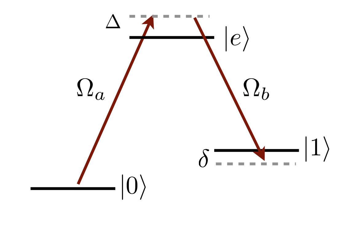
Parameters:

• Pa – power (W), of laser a \(\vert 0 \rangle\rightarrow\vert e\rangle\)

• wa – beam waist (m) of laser a \(\vert 0 \rangle\rightarrow\vert e\rangle\)

• qa – polarisation (+1, 0 or -1 corresponding to driving \(\sigma^+\), \(\pi\) and \(\sigma^-\)) of laser a \(\vert 0 \rangle\rightarrow\vert e\rangle\)

• Pb – power (W) of laser b \(\vert 1 \rangle\rightarrow\vert e\rangle\)

• wb – beam waist (m) of laser b \(\vert 1 \rangle\rightarrow\vert e\rangle\)

• qb – polarisation (+1, 0 or -1 corresponding to driving \(\sigma^+\), \(\pi\) and \(\sigma^-\)) of laser b \(\vert 1 \rangle\rightarrow\vert e\rangle\)

• Delta – Detuning from excited state centre of mass (rad \(\mathrm{s}^{-1}\))

• f0 – Lower hyperfine level

• mf0 – Lower hyperfine level

• f1 – Upper hyperfine level

• mf1 – Upper hyperfine level

• ne – principal, orbital, total orbital quantum numbers of excited state

• le – principal, orbital, total orbital quantum numbers of excited state

• je – principal, orbital, total orbital quantum numbers of excited state

Returns:

Two-Photon Rabi frequency \(\Omega_R\) (units \(\mathrm{rads}^{-1}\)), differential AC Stark shift \(\Delta_\mathrm{AC}\) (units \(\mathrm{rads}^{-1}\)) and probability to scatter a photon during a \(\pi\)-pulse \(P_\mathrm{sc}\)

Return type:

float

hyperfineStructureData: str = ''

file cotaining data on hyperfine structure (magnetic dipole A and magnetic quadrupole B constnats).

ionisationEnergy = 13.598433

ionisationEnergy in eV

levelDataFromNIST: str = ''

file with .csv data, each row is [n, l, s, j, energy, source, absolute uncertanty]

literatureDMEfilename: str = ''

Filename of the additional literature source values of dipole matrix elements. These additional values should be saved as reduced dipole matrix elements in J basis.

mass: float = 0.0

atomic mass in kg

minQuantumDefectN: int = 0

Not used with DivalentAtom, see defectFittingRange instead.

modelPotential_coef: dict = {}

Model potential parameters fitted from experimental observations for different l (electron angular momentum)

potential(l, s, j, r)

Not implemented for Alkaline earths

quadrupoleMatrixElementFile: str = ''

location of hard-disk stored dipole matrix elements

quantumDefect = [[[0.0, 0.0, 0.0, 0.0, 0.0, 0.0], [0.0, 0.0, 0.0, 0.0, 0.0, 0.0], [0.0, 0.0, 0.0, 0.0, 0.0, 0.0], [0.0, 0.0, 0.0, 0.0, 0.0, 0.0], [0.0, 0.0, 0.0, 0.0, 0.0, 0.0]], [[0.0, 0.0, 0.0, 0.0, 0.0, 0.0], [0.0, 0.0, 0.0, 0.0, 0.0, 0.0], [0.0, 0.0, 0.0, 0.0, 0.0, 0.0], [0.0, 0.0, 0.0, 0.0, 0.0, 0.0], [0.0, 0.0, 0.0, 0.0, 0.0, 0.0]], [[0.0, 0.0, 0.0, 0.0, 0.0, 0.0], [0.0, 0.0, 0.0, 0.0, 0.0, 0.0], [0.0, 0.0, 0.0, 0.0, 0.0, 0.0], [0.0, 0.0, 0.0, 0.0, 0.0, 0.0], [0.0, 0.0, 0.0, 0.0, 0.0, 0.0]], [[0.0, 0.0, 0.0, 0.0, 0.0, 0.0], [0.0, 0.0, 0.0, 0.0, 0.0, 0.0], [0.0, 0.0, 0.0, 0.0, 0.0, 0.0], [0.0, 0.0, 0.0, 0.0, 0.0, 0.0], [0.0, 0.0, 0.0, 0.0, 0.0, 0.0]]]

Contains list of modified Rydberg-Ritz coefficients for calculating quantum defects for [[ \(^1S_{0},^1P_{1},^1D_{2},^1F_{3}\)], [ \(^3S_{0},^3P_{0},^3D_{1},^3F_{2}\)], [ \(^3S_{0},^3P_{1},^3D_{2},^3F_{3}\)], [ \(^3S_{1},^3P_{2},^3D_{3},^3F_{4}\)]].

radialWavefunction(l, s, j, stateEnergy, innerLimit, outerLimit, step)

Not implemented for Alkaline earths

sEnergy: NDArray = array([], dtype=float64)

state energies from NIST values sEnergy [n,l] = state energy for n, l, j = l-1/2 sEnergy [l,n] = state energy for j = l+1/2

twoPhotonRydbergExcitation(Pp: float, wp: float, qp: int, Pc: float, wc: float, qc: int, Delta: float, fg: int, mfg: int, ne: int, le: int, je: float, nr: int, lr: int, jr: float, mjr: float) → Tuple[ndarray[Any, dtype[_ScalarType_co]], ndarray[Any, dtype[_ScalarType_co]], ndarray[Any, dtype[_ScalarType_co]], ndarray[Any, dtype[_ScalarType_co]]]

Returns two-photon Rabi frequency \(\Omega_R\), ground AC Stark shift \(\Delta_{\mathrm{AC}_g}\), Rydberg state AC Stark shift \(\Delta_{\mathrm{AC}_r}\) and probability to scatter a photon during a \(\pi\)-pulse \(P_\mathrm{sc}\) for two-photon excitation from \(\vert f_h,m_{f_g}\rangle\rightarrow \vert j_r,m_{j_r}\rangle\) via intermediate excited state

\(\Omega_R=\displaystyle\sum_{f_e,m_{f_e}}\frac{\Omega_p^{g\rightarrow f_e}\Omega_c^{f_e\rightarrow r}}{2(\Delta-\Delta_{f_e})}\)

\(\Delta_{\mathrm{AC}_g} = \displaystyle\sum_{f_e,m_{f_e}}\frac{\vert\Omega_p^{g\rightarrow f_e}\vert^2}{4(\Delta-\Delta_{f_e})}\)

\(\Delta_{\mathrm{AC}_r} = \displaystyle\sum_{f_e,m_{f_e}}\frac{\vert\Omega_p^{g\rightarrow f_e}\vert^2}{4(\Delta-\Delta_{f_e})}`\)

\(P_\mathrm{sc} = \frac{\Gamma_et_\pi}{2}\displaystyle\sum_{f_e,m_{f_e}}\left[\frac{\vert\Omega_p^{g\rightarrow f_e}\vert^2}{2(\Delta-\Delta_{f_e})^2}+\frac{\vert\Omega_c^{f_e\rightarrow r}\vert^2}{2(\Delta-\Delta_{f_e})^2}\right]\)

where \(\tau_\pi=\pi/\Omega_R\).

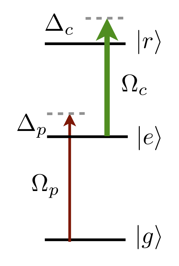
Parameters:

• Pp – power (W) of probe laser \(\vert g \rangle\rightarrow\vert e\rangle\)

• wp – beam waist (m) of probe laser \(\vert g \rangle\rightarrow\vert e\rangle\)

• qp – polarisation (+1, 0 or -1 corresponding to driving \(\sigma^+\),:math:pi and \(\sigma^-\)) of probe laser \(\vert g \rangle\rightarrow\vert e\rangle\)

• Pb – power (W) of coupling laser \(\vert e\rangle\rightarrow\vert r\rangle\)

• wb – beam waist (m) of coupling laser \(\vert e\rangle\rightarrow\vert r\rangle\)

• qb – polarisation (+1, 0 or -1 corresponding to driving \(\sigma^+\),:math:pi and \(\sigma^-\)) of coupling laser \(\vert e\rangle\rightarrow\vert r\rangle\)

• Delta – Detuning from excited state centre of mass (rad s:math:^{-1})

• fg – ground state hyperfine state

• mfg – projection of ground state hyperfine state

• f1 – upper hyperfine state

• mf1 – upper hyperfine state

• ne – principal quantum numbers of excited state

• le – orbital angular momentum of excited state

• je – total angular momentum of excited state

• nr – principal quantum number of target Rydberg state

• lr – orbital angular momentum of target Rydberg state

• jr – total angular momentum of target Rydberg state

• mjr – projection of total angular momenutm of target Rydberg state

Returns:

Two-Photon Rabi frequency \(\Omega_R\) (units \(\mathrm{rads}^{-1}\)), ground-state AC Stark shift \(\Delta_{\mathrm{AC}_g}\) (units \(\mathrm{rads}^{-1}\)) Rydberg-state AC Stark shift \(\Delta_{\mathrm{AC}_r}\) (units \(\mathrm{rads}^{-1}\)) and probability to scatter a photon during a \(\pi\)-pulse \(P_\mathrm{sc}\)

Return type:

float

updateDipoleMatrixElementsFile()

Updates the file with pre-calculated dipole matrix elements.

This function will add the the file all the elements that have been calculated in the previous run, allowing quick access to them in the future calculations.

update_me_cache()

Updates cached dipole and quadrupole matrix elements saved in ~/.arc-data